2 easy ways to remove gridlines in Excel

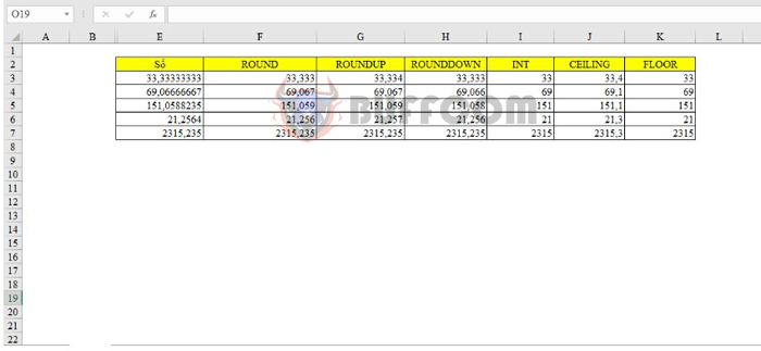
Gridlines are the default lines in Excel that divide cells. However, sometimes they can be annoying and distracting. So how can you remove gridlines in Excel? Let’s explore two simple and quick ways to remove gridlines in Excel.

Method 1: Remove all gridlines except for the table

Suppose you want to remove gridlines outside the table range. You can follow one of the two methods below:

2 easy ways to remove gridlines in Excel

Method 1:

On the toolbar, select the View tab. Then uncheck the box next to Gridlines under the Show section.

2 easy ways to remove gridlines in Excel

The gridlines will disappear, and the result will be displayed as follows:

2 easy ways to remove gridlines in Excel

Method 2:

Besides Method 1, you can also remove gridlines by following these steps:
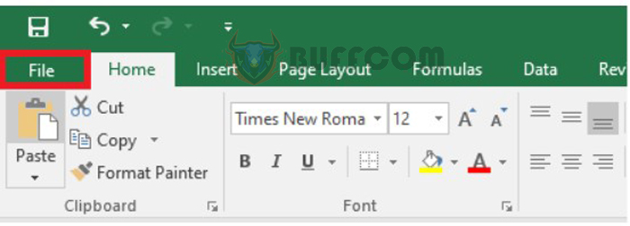
On the toolbar, select the File tab, then select Options.

2 easy ways to remove gridlines in Excel

Select Options.

2 easy ways to remove gridlines in Excel

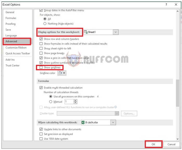
Excel Options will appear. Select the Advanced tab. Under Display options for this worksheet, uncheck the box next to Show gridlines as shown in the illustration below.

2 easy ways to remove gridlines in Excel

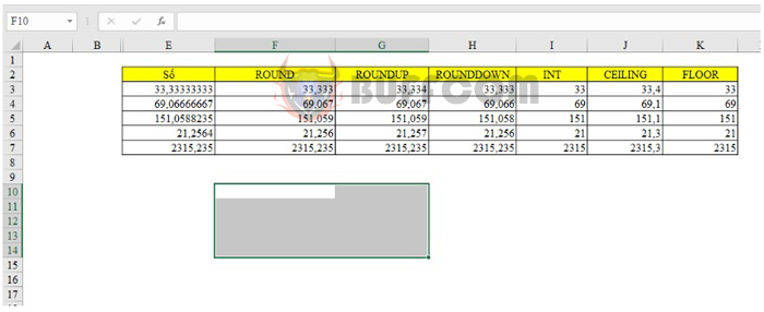
Then click OK to finish. Similar to Method 1, all gridlines outside the table will be removed, and the worksheet will be displayed as follows:

2 easy ways to remove gridlines in Excel

Method 2: Remove gridlines in a specific range

If you only want to remove gridlines in a certain range, follow these two steps:

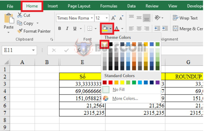
Step 1: Select the range where you want to remove gridlines.
Step 2: On the toolbar, select the Home tab. Look for the paint bucket icon under the Font section of this tab. Click the paint bucket icon and choose the color white.

2 easy ways to remove gridlines in Excel

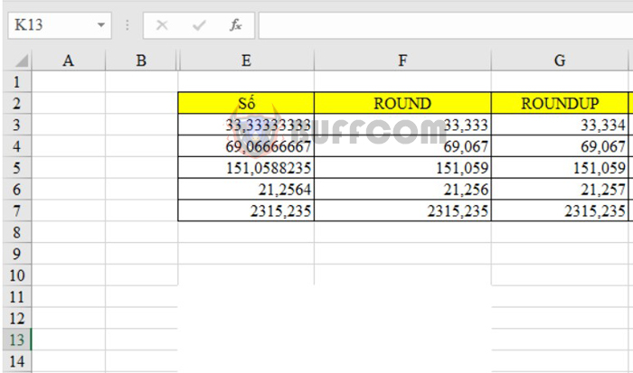
The selected range will be filled with white, as shown below.

2 easy ways to remove gridlines in Excel

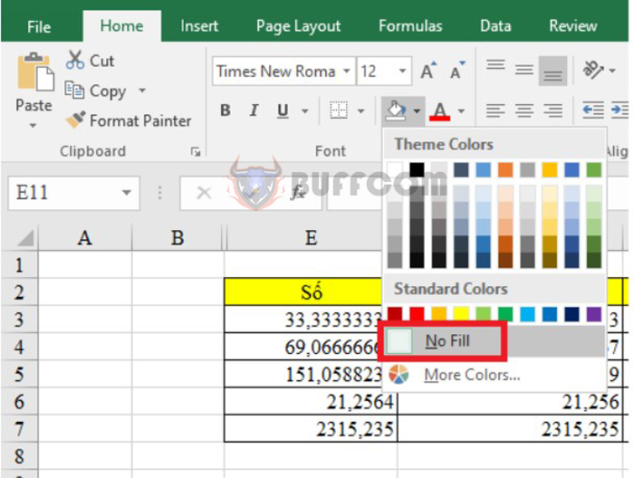
If you want to restore gridlines in this area, just select the paint bucket icon again and check the box next to No Fill.

With these basic steps, you can easily remove gridlines in Excel. Good luck!