3 simple ways to round numbers in Excel using the ROUND function
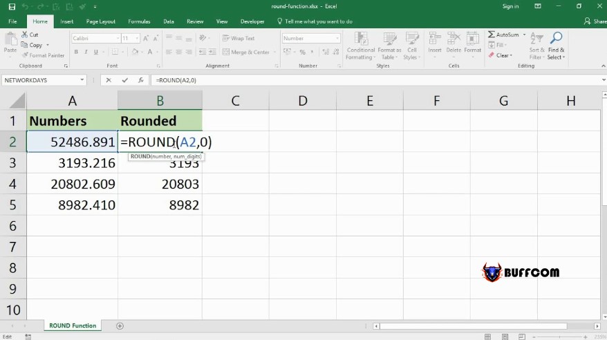
If you often work with numerical data in Excel and encounter decimal numbers with odd digits after the decimal point, don’t worry. In this article, we will show you three simple ways to round numbers using the ROUND function in Excel.
Rounding numbers in Excel is very simple, requiring only a few small steps. If you want to round numbers in Excel and remove decimal values, you can use three built-in functions: ROUND, ROUNDUP, and ROUNDDOWN. Let’s let Buffcom.net explain and guide you on how to use these functions.
 Using the ROUND functions in Excel is different from changing the format of a number. When you change the format of a number, you only change its appearance in the worksheet, but the underlying value remains unchanged. In contrast, when you use the ROUND function, Excel helps you round numbers as desired.
The ROUND function rounds a number to a specified number of decimal places. It rounds down if the digit to the right of the decimal point is between 0 and 4, and it rounds up if that digit is between 5 and 9. As the name implies, the ROUNDUP function always rounds up, while the ROUNDDOWN function always rounds down.
1. How to round numbers up using the ROUND function in Excel
The ROUND function rounds a number to a specified decimal place that you configure. If the digit to the right is between 0 and 4, it rounds down. Therefore, for example, if you round the number 8.532 using the ROUND function, it will become 8.53. If the digit to the right is between 5 and 9, it rounds up. Therefore, 8.538 will become 8.54. The ROUND function can round numbers to the left or right of the decimal point as desired.
You can apply formatting to blank cells or cells that already have numbers. You can also use ROUND as part of a more complex formula if desired. For example, you can create a formula that adds two columns together using the SUM function, and then round the result.
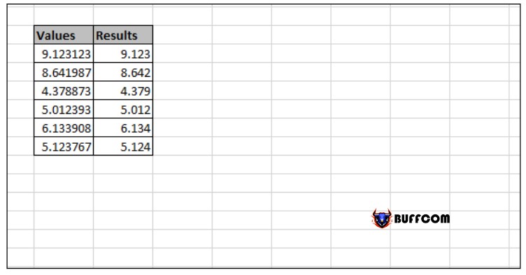
For this example, we have a column of numbers called “Values” that contains our random natural numbers. The column to the right is the “Result” column, where we will place the rounded values to the second decimal place.
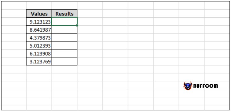
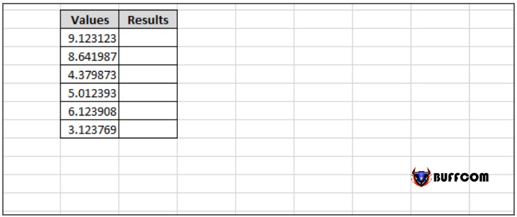 Step 1: Select the cell that you want to round.
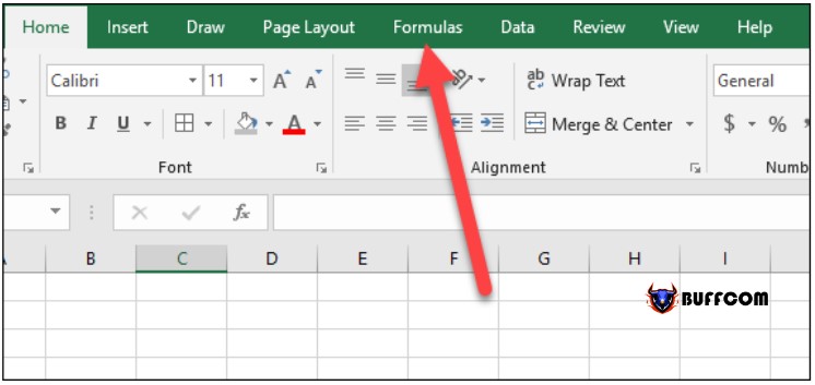
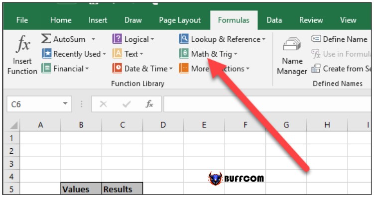
 Step 2: Click on the “Formulas” tab in the top navigation bar.
Step 3: Once the Formulas tab opens, click on “Math & Trig”.
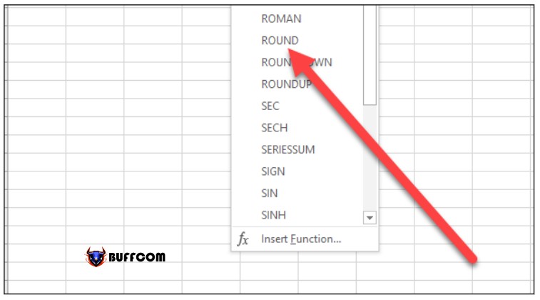
 Step 4: Under the “Math & Trig” dropdown menu, click on the “ROUND” function.
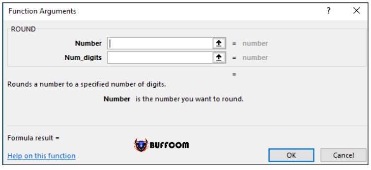
 Step 5: A new window will open, inside of which are the options for the ROUND function that you can customize as desired.
 Step 6: Use the “Number” field for the number, cell, column or row you want to round. You can round a number entered directly into it, but typically, we use Excel by calling a number from an existing cell in our spreadsheet. Here, we are using B6 as the value at the top of the “Values” column.
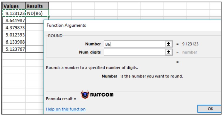 Step 7: Use the “Num_Digits” field to choose how many decimal places to round to. Refer to the following:
Use a positive integer (such as n) to round to the nth decimal place. For example, entering “3” will round to the third decimal place to the right of the decimal point.
Enter “0” to round to the nearest integer.
Use a negative integer (such as -n) to round to the nth digit to the left of the decimal point. For example, if you round the number 328.25 and enter “-1” here, it will round your number to 330.
In our example, we are entering “3” to round our result to the third decimal place to the right of the decimal point.
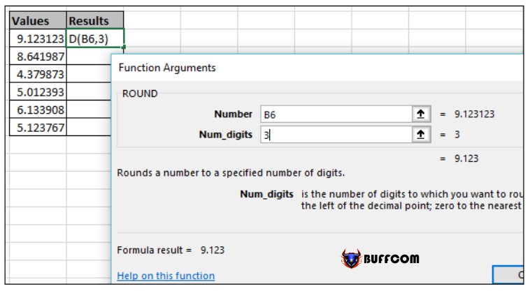 Step 8: After completing the options, click “OK” to finish.
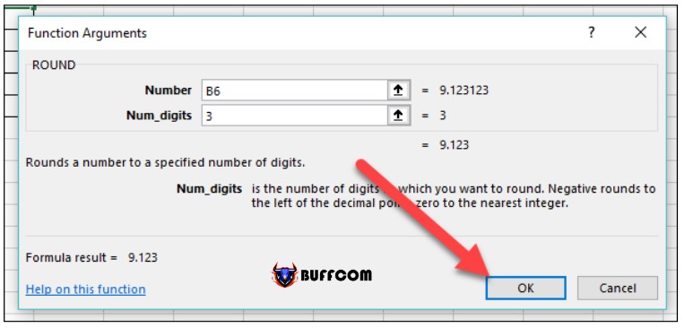 As shown in the image below, the rounded result of cell B6 has been rounded to the third decimal place in the cell we selected, here we have chosen the top cell of the “Results” column.
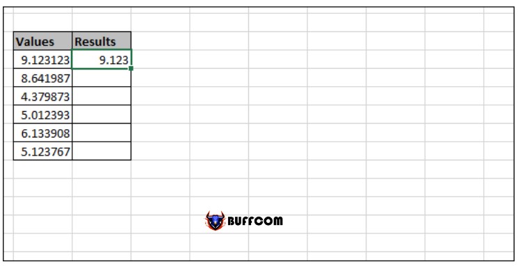 Step 9: You can use the formula of the ROUND function you just entered for the cells below by clicking and holding the blue dot in the lower right corner of the cell you want to copy, then dragging it to the cell you want.
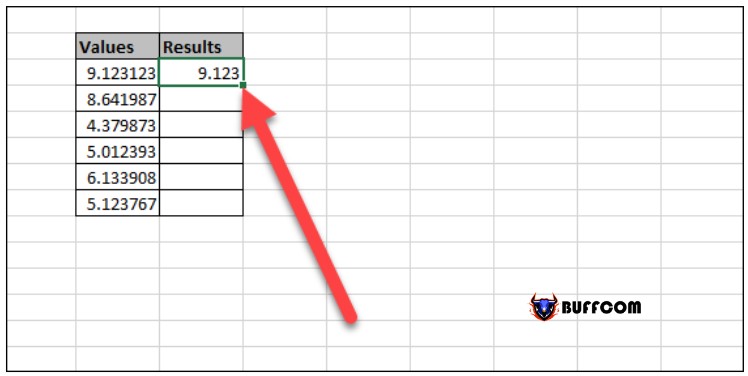 All the cells you select will change values just like the cell you selected after completing the above steps. You can also copy the formula in the cell you want to copy and paste it into the cell you want to use the same formula in Excel.
 You can also do all of this just by using Excel’s Function bar if you want.
Step 1: Select the column that you want the numbers to be rounded in.
Step 2: Click on the Function bar to enter the function you want on it.
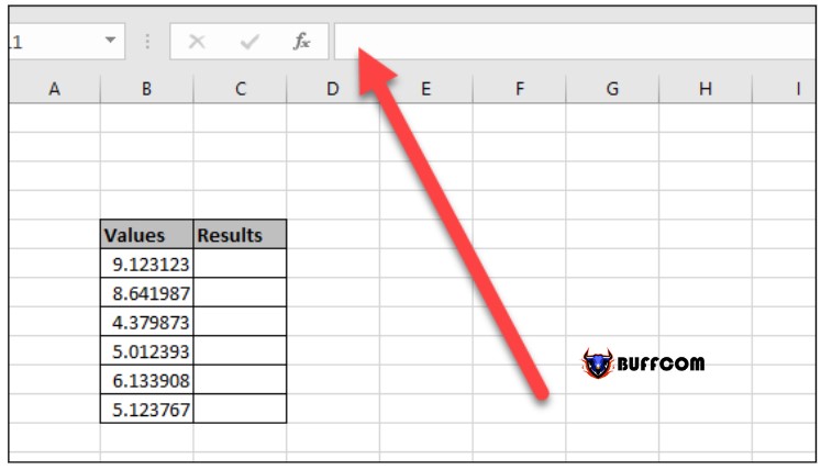 Step 3: Type “ROUND” and select it from the drop-down menu.
Step 4: Enter your formula using the syntax:
= ROUND(number, num_digits)
Where “number” is the cell or number you want to round and “num_digits” determines to which decimal place you want to round.
For example, here’s how we entered the same rounding formula we applied earlier using the dialog box.
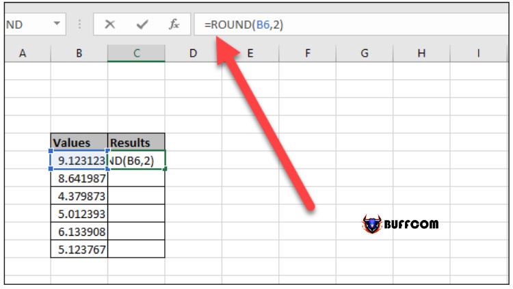 Press Enter (or Return) after entering your formula, and your number is now rounded.
2. Rounding Numbers in Excel with ROUNDUP or ROUNDDOWN function
Sometimes, you may want your numbers to only round up or down instead of depending on the next digit of the number you want to round. That’s what the ROUNDUP and ROUNDDOWN functions can help you do.
Click on the cell that you want your result to be rounded in.
Go to Formulas > Math & Trig, and then select the “ROUNDUP” or “ROUNDDOWN” function from the drop-down menu.
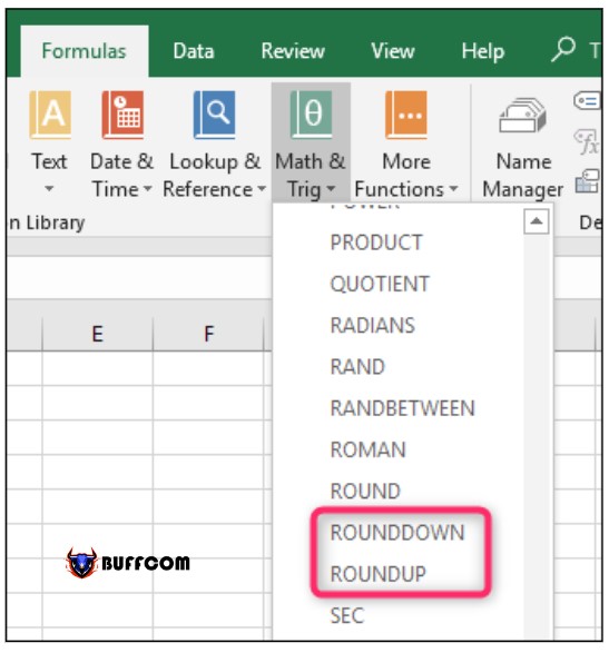 Enter the number (or cell) you want to round into the “Number” field. Enter the number of decimal places you want to round to into the “Num_digits” field. The same rounding rules apply as with the ROUND function. A positive integer rounds to the right of the decimal point, zero rounds to the nearest integer, and a negative integer rounds to the left of the decimal point.
Click “OK” when you’ve set everything up.
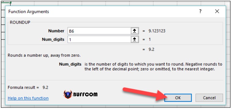 And just like with the ROUND function, you can also set up the ROUNDUP and ROUNDDOWN functions by typing them into the Function bar, and you can use them as part of more complex formulas.
That’s how to use the ROUND functions to round numbers in Excel. It’s really simple, isn’t it? If you have any questions or comments about the article, please leave a comment for Buffcom.net to answer. Thank you for reading the article.


