Combining VLOOKUP and MATCH Functions to Retrieve Results from Multiple Columns
Combining VLOOKUP and MATCH Functions to Retrieve Results from Multiple Columns: The VLOOKUP function is widely used in Excel. To maximize its potential, you can combine it with other functions to enhance flexibility in searching without directly modifying the formula. One common scenario is combining the VLOOKUP and MATCH functions to retrieve results from multiple columns. For example, when searching for monthly revenues, prices, quantities, etc. Read the following article to learn how to achieve this.
Problem:
The goal of combining VLOOKUP and MATCH functions is to avoid directly modifying the formula while referencing with multiple conditions. Here, the conditions are the lookup position and the number of columns to reference, which may vary. Let’s solve the problem below:
Determine the revenue for each month (from month 1 to month 3) based on the selected selling price in cell E1.
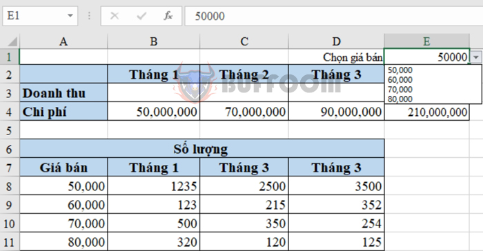
For this scenario, we’ll use the VLOOKUP function to reference the quantity sold for each month, and then calculate revenue using the formula: Revenue = Selling Price × Quantity.
First, let’s understand the structures of the VLOOKUP and MATCH functions.
VLOOKUP Function Structure
The VLOOKUP function searches for data in Excel. Its syntax is as follows:
=Vlookup(lookup_value,table_array,col_index_num,[range_lookup])
Where:
Lookup_value: the value to search for. In this scenario, it’s the selected selling price in cell E1.
Table_array: the range containing the values to be searched. This should be in absolute reference format using “$” before the column and row labels. The first column in the table_array contains the search value. For this problem, the table_array is $A$7:$D$11.
Col_index_num: the index of the column containing the search value within the table_array.
Range_lookup: the search range. TRUE corresponds to 1 (approximate match), FALSE corresponds to 0 (exact match). This parameter is optional. For this problem, we choose 0 (exact match).
So, only the col_index_num parameter varies based on the result column position. To avoid manual entry, we can determine col_index_num using the MATCH function.
MATCH Function Structure
The MATCH function searches for a specified value within a range and returns its position within that range.
For instance, when calculating the revenue for month 1 using VLOOKUP, we need to determine the corresponding column for month 1 in the range A7:D11 to find col_index_num. This is equivalent to determining the position of “Month 1” within the header row. This will be used in the formula to determine where B2 corresponds within the range A7:D7.
The structure of the MATCH function:
=Match(lookup_value,lookup_array,[match_type])
Where:
Lookup_value: the value to search for. In this scenario, the lookup values are the month names, which are B2, C2, D2.
Lookup_array: the range to search within. For this problem, the search range is A7:D7.
Match_type: the matching method, exact or approximate. For this problem, we need an exact match, so match_type is 0.
Combining VLOOKUP and MATCH
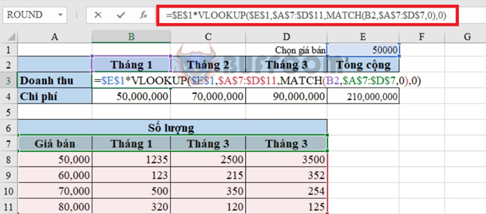
By combining these two functions, we can calculate the revenue in cell B3 with E1 = 50,000 (revenue for month 1 with a selling price of 50,000) as follows:
=$E$1*VLOOKUP($E$1,$A$7:$D$11,MATCH(B2,$A$7:$D$7,0),0)
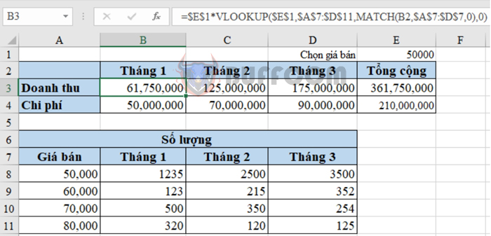
 After copying the formula to adjacent cells, the results will be as shown:
Combining VLOOKUP and MATCH Functions to Retrieve Results from Multiple Columns
If you want to calculate revenues for different months at different price levels, you can select the price in cell E1. The table below demonstrates revenues for a price of 60,000.
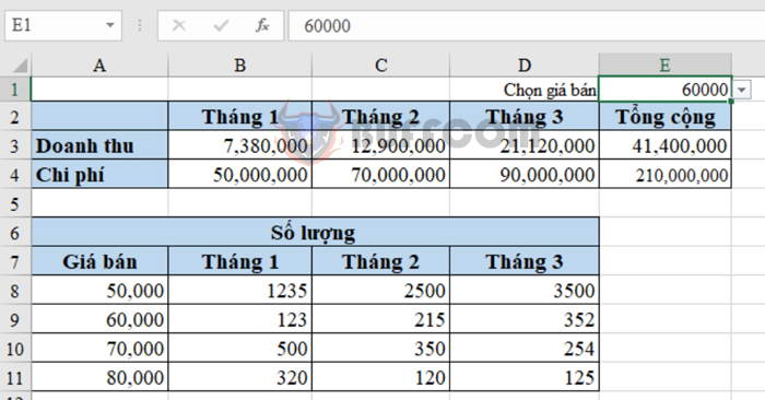 The above method showcases how to use the combination of VLOOKUP and MATCH functions to retrieve results from multiple columns. Feel free to refer to and apply this technique. Best of luck!

