How to Create a Dropdown List with Hyperlinks to Sheets
How to Create a Dropdown List with Hyperlinks to Sheets. In the previous article, I guided you on how to create an automatic table of contents for sheets in Excel and received very positive feedback. Today, I will introduce you to another way to quickly and easily navigate to sheets – creating a dropdown list with hyperlinks to sheets.
Get all sheet names
How to Create a Dropdown List with Hyperlinks to Sheets
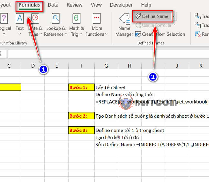
First, we need to get the names of all sheets currently in the workbook for use in the dropdown list. First, we need to define a formula by selecting Define Name in the Formulas tab.
How to Create a Dropdown List with Hyperlinks to Sheets
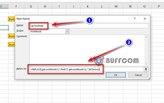
At this point, the New Name dialog box appears. In the Name field, you enter a formula name that is easy to remember and use later. In the example below, the formula is used to get the names of the current sheets, so I named it LayTenSheet. In the Refers to field, you enter =REPLACE(get.workbook(1),1,find(“]”,get.workbook(1)),””)&T(now()).
How to Create a Dropdown List with Hyperlinks to Sheets
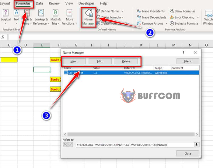
For convenience in managing formulas, in the Formulas tab, you can select Name Manager. In the Name Manager dialog box, there are 3 main buttons at the top: New, Edit, and Delete, with corresponding functions to create a new formula, edit a formula, and delete a formula. Below will display all the formulas you have created previously.
How to Create a Dropdown List with Hyperlinks to Sheets
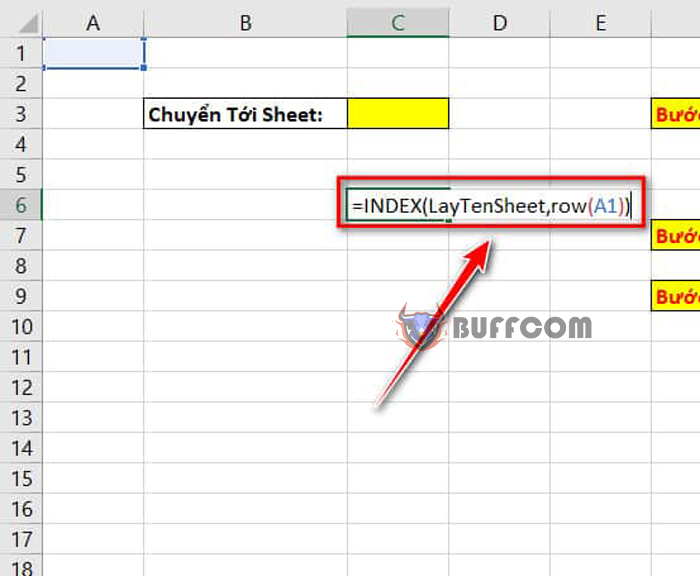
After defining the formula to retrieve the sheet name, you can retrieve the name values of the sheets into cells by entering “=INDEX(GetSheetName,ROW(A1))” into any cell. In the INDEX function, we pass two parameters: the name of the formula we just created and the row index.
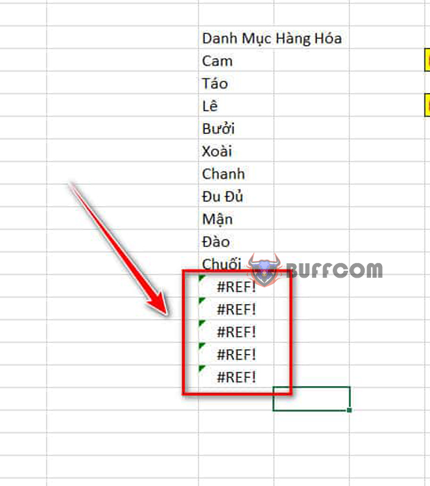
Next, you can drag the formula down to apply it to other cells. Note that if you drag it too far, some cells will have a value of #REF!. This is because the previous values have already retrieved all the sheet names, so the subsequent values will not have any names to retrieve. You can simply select these error values and press the Delete button on your keyboard.
Creating a dropdown list
How to Create a Dropdown List with Hyperlinks to Sheets
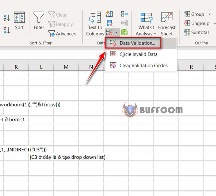
The next step is to create a dropdown list with the sheet names that we retrieved. First, select the cell where you want to create the dropdown list (in my example, it’s cell C3), then go to the Data tab and select Data Validation.
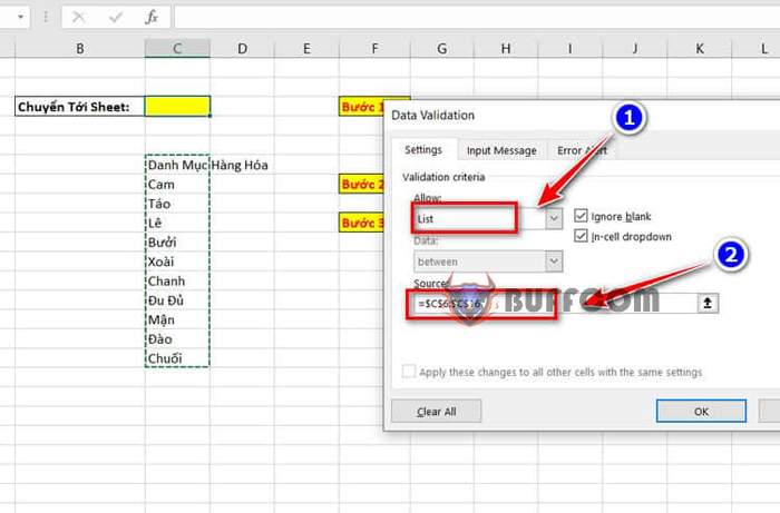
In the Data Validation dialog box, change the Allow option to List (the default value is Any value). In the Source field, select the data range that contains the sheet names.
Creating links to the sheets
How to Create a Dropdown List with Hyperlinks to Sheets
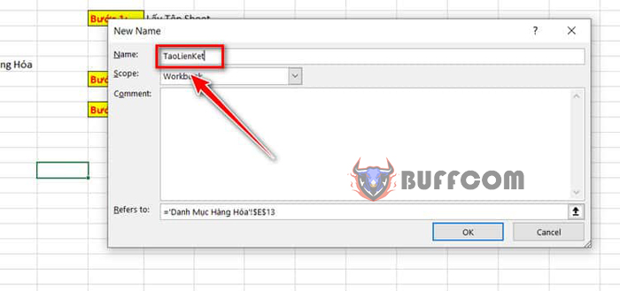
After successfully creating the dropdown list, the next step is to create links to switch to those sheets. Similar to how we created the formula to retrieve the sheet name in the first step, go to the Formulas tab and select Define Name. Then enter the name of the formula as “CreateLink” and click OK.
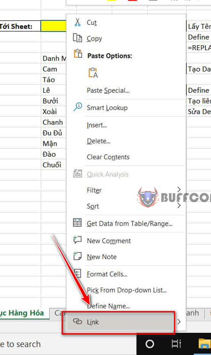
Right-click on the cell that contains the dropdown list, and select Link to create a link to the corresponding sheet.
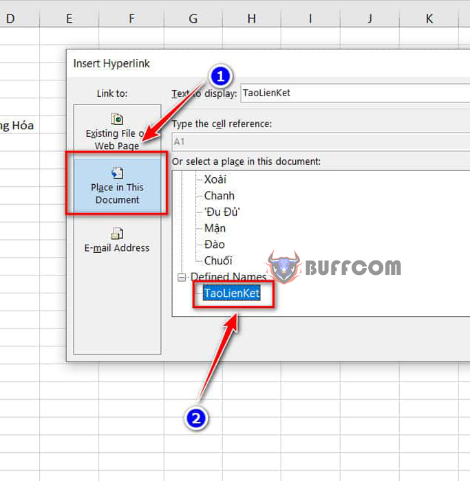
In the Insert Hyperlink dialog box, under the Link to section, choose “Place in This Document”, then scroll down and select the name of the formula you just created (TaoLienKet). At this point, when you click on any value in the dropdown list, it will refer to a cell in the sheet instead of other sheets. Therefore, we need to adjust the TaoLienKet formula a bit.
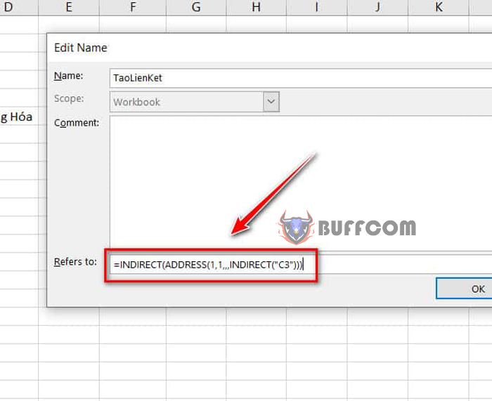
In the Formulas tab, select “Name Manager”, choose the TaoLienKet formula, and click on the “Edit” button to make the necessary adjustments. Next, in the “Refers to” field, enter =INDIRECT(ADDRESS(1,1,,,INDIRECT(“C3”))). Note that the cell C3 in the INDIRECT function is the cell that contains your dropdown list. Buffcom wish you all the best in practicing this!


