How to use the NOT function and combine it with other logic functions in Excel

How to use the NOT function and combine it with other logic functions in Excel: The NOT function is one of the basic logic functions widely used in Excel. It returns the opposite value of a known result. For example, if you have a large data table and want to find values greater than 500, the NOT function helps you identify which data is either “True” or “False”. In this article, Buffcom.net will introduce you to the details of how to use the NOT function and how to combine it with other logic functions.
1. Function structure
Function syntax: =NOT(logical)
Where “logical” is a value or logical proposition.
Note:
- The NOT function returns the opposite value of a given value or logical proposition.
- If the logical proposition is TRUE, the NOT function returns FALSE.
- If the logical proposition is FALSE, the NOT function returns TRUE.
2. How to use the NOT function
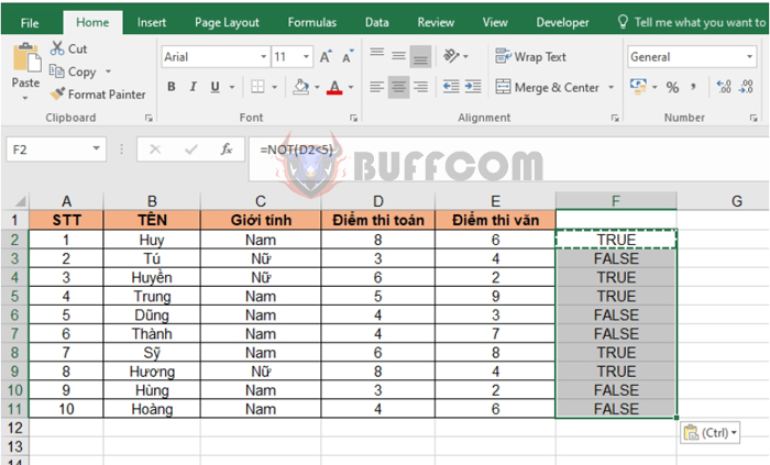
For example, suppose you have a table of math and literature scores for students as shown in the image below.

To find students with math scores greater than or equal to 5, you can use the formula in cell F2 as follows:
=NOT(D2<5)
Copy the formula for all students to obtain the results of students with math scores greater than 5 as TRUE and those with math scores less than 5 as FALSE.

How to use the NOT function and combine it with other logic functions in Excel
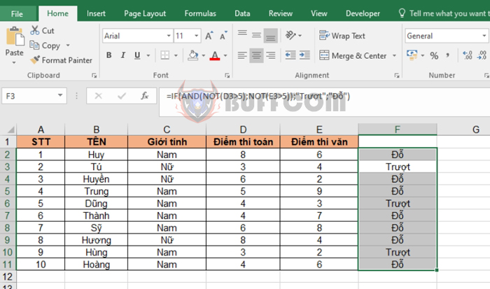
You can also use the NOT function in combination with other logic functions like AND and IF for calculation. For example, if a student has both math and literature scores less than 5, they fail; otherwise, they pass. You can use the following formula:
=IF(AND(NOT(D2>5),NOT(E2>5)),”Fail”,”Pass”)
Copy the formula for all students to get the result that three students, Tu, Dung, and Hung, fail because they have both math and literature scores less than 5.

How to use the NOT function and combine it with other logic functions in Excel
In conclusion, this article has guided you on how to use the NOT function and how to combine it with IF and AND functions in Excel. Good luck!


