Using IFERROR with VLOOKUP in Excel to Handle #N/A Errors
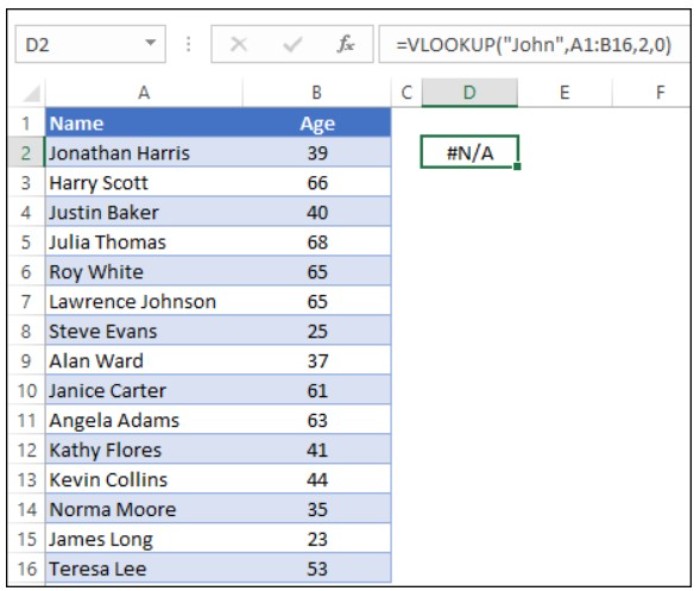
When using VLOOKUP in Excel, if the value you are searching for is not present in the data, you will receive a #N/A error. This occurs because VLOOKUP is unable to find the value you are searching for.
Using IFERROR with VLOOKUP in Excel to Handle #N/A Errors
To handle this error and make it easier for others to understand, you can replace #N/A with a custom value. The best way to do this is by using the IFERROR function with VLOOKUP.
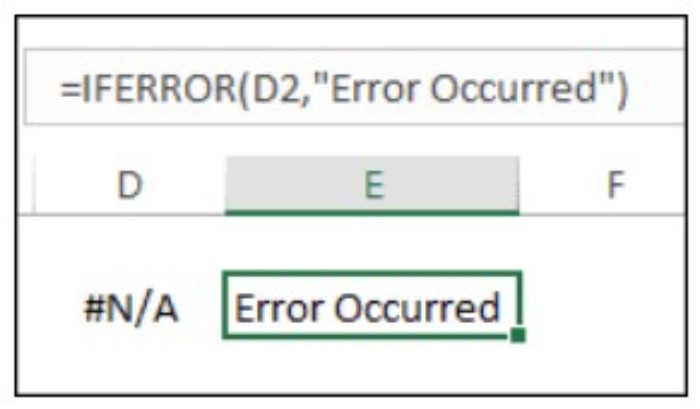
IFERROR is a function that allows you to evaluate a value and return a custom value if that value results in an error. The syntax for IFERROR is as follows:
IFERROR(value, value_if_error)
Here, you need to provide two arguments. The first argument is the value you want to evaluate, and the second argument is the custom value you want to return if an error occurs.
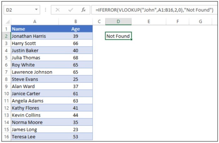
To use IFERROR with VLOOKUP, simply replace the value argument in IFERROR with your VLOOKUP formula. For the value_if_error argument, specify the value you want to return whenever VLOOKUP returns #N/A.
For example, if you are searching for the name “John” in a list of employees and it is not present, VLOOKUP will return #N/A.
Using IFERROR with VLOOKUP in Excel to Handle #N/A Errors
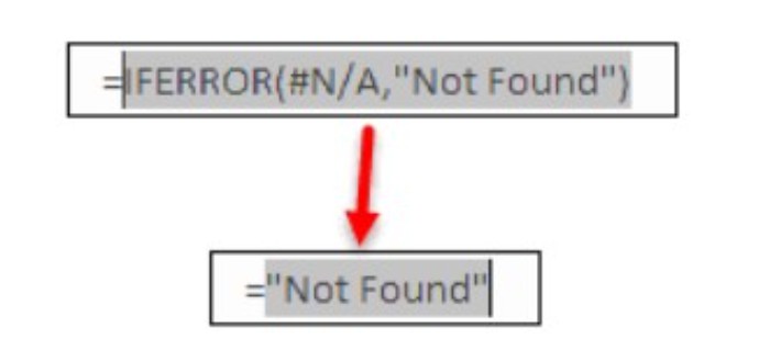
By using IFERROR with VLOOKUP and specifying “Not Found” as the value_if_error argument, all cells with #N/A errors will return “Not Found” instead.
Replacing #N/A with IFERROR in VLOOKUP in Excel
Whenever the value you are looking for is not present in the data, VLOOKUP returns a #N/A error. This error can be replaced with a custom value to make it more understandable. One way to replace the #N/A error is to use IFERROR with VLOOKUP. IFERROR is a function that evaluates a value, and if that value is an error, it returns a custom value instead of the error.
To use IFERROR with VLOOKUP, you need to specify two things in the IFERROR function – the value you want to evaluate and a custom value to return whenever an error occurs. The syntax for IFERROR is as follows:
IFERROR(value, value_if_error)
Using IFERROR with VLOOKUP in Excel to Handle #N/A Errors
In this combination, VLOOKUP works first, looking up a value and returning the result value if found, otherwise an error. IFERROR then evaluates the result of VLOOKUP. If the result is an error, IFERROR replaces that error with the custom value you have specified. Otherwise, it returns the same result as VLOOKUP.
It’s important to note that IFERROR replaces the value for all types of errors. So, you will get the same custom value for all errors. If there is any chance of getting an error other than #N/A, you can use IFNA instead of IFERROR. IFNA only evaluates #N/A.
In older versions of Excel where IFERROR is not available, you can replace #N/A with a custom value by combining IF and ISNA with VLOOKUP. The formula for this is:
=IF(ISNA(VLOOKUP(A1,table,2,FALSE)),”Not Found”,VLOOKUP(A1,table,2,FALSE))
Using IFERROR with VLOOKUP in Excel to Handle #N/A Errors
In this formula, VLOOKUP is evaluated with ISNA (which only evaluates #N/A and returns TRUE). When VLOOKUP returns an error, IFNA converts it into TRUE.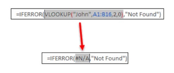 IF then returns the value specified for TRUE, otherwise, the value for FALSE is the same VLOOKUP formula.
In conclusion, it’s recommended to use IFERROR with VLOOKUP to replace #N/A errors as it makes the data more understandable. Numeric values with errors cannot be used, so it’s best to replace the error with a custom value like “0”.


