5 Great Tips for Google Sheets Users to Know

Are you struggling with Google Sheets? Do you find it difficult to manipulate data in Google Sheets? Don’t worry, in this article, I will guide you through 5 great tips in Google Sheets that users should know. Let’s Buffcom.net explore them below!
Tip 1: Use Sparkline to insert small graphs
Sometimes, you may be dealing with a lot of numbers and you know that when working in a spreadsheet, you have rows and columns of numbers. Sometimes it’s hard to visualize extremely long numbers. Of course, you can create a chart in Google Sheets. But sometimes a chart is too much and you don’t want to use this large chart in your spreadsheet. You just want to quickly see the data that is happening in the spreadsheet. A great tip to help you do that is with the smart feature Sparkline.
The steps are as follows:
Step 1: Select any cell to display the Sparkline chart location.
Step 2: Type: =SPARKLINE(D2:D17)
Explanation: D2:D17: The range of data to analyze.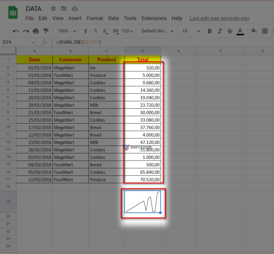
Tip 2: Share comments and notifications directly with others
Do you want to comment or add your opinion to the data so that everyone knows? It’s great that in Google Sheets, there is a feature that helps you do that. You just need to follow these steps:
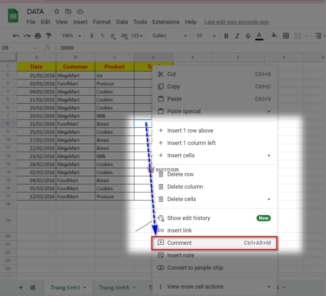
First, at the cell where you want to insert a comment, right-click and select the Comment feature.
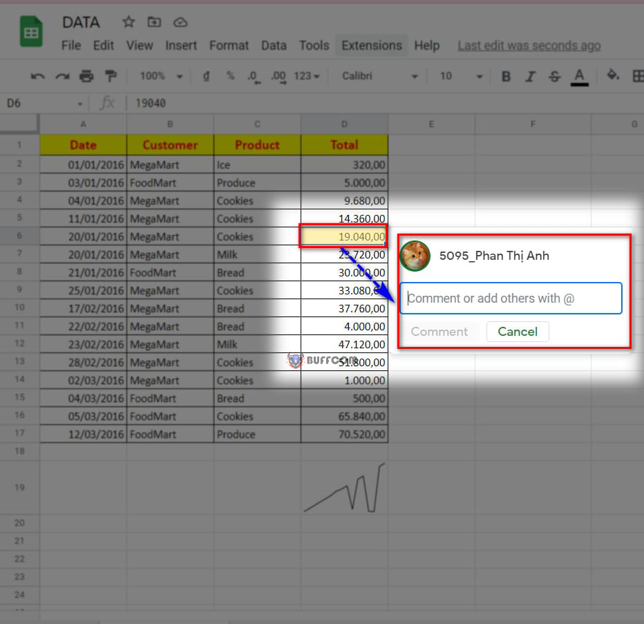
 A box containing the comment will appear. Here, you can write what you want to comment or add to the data.
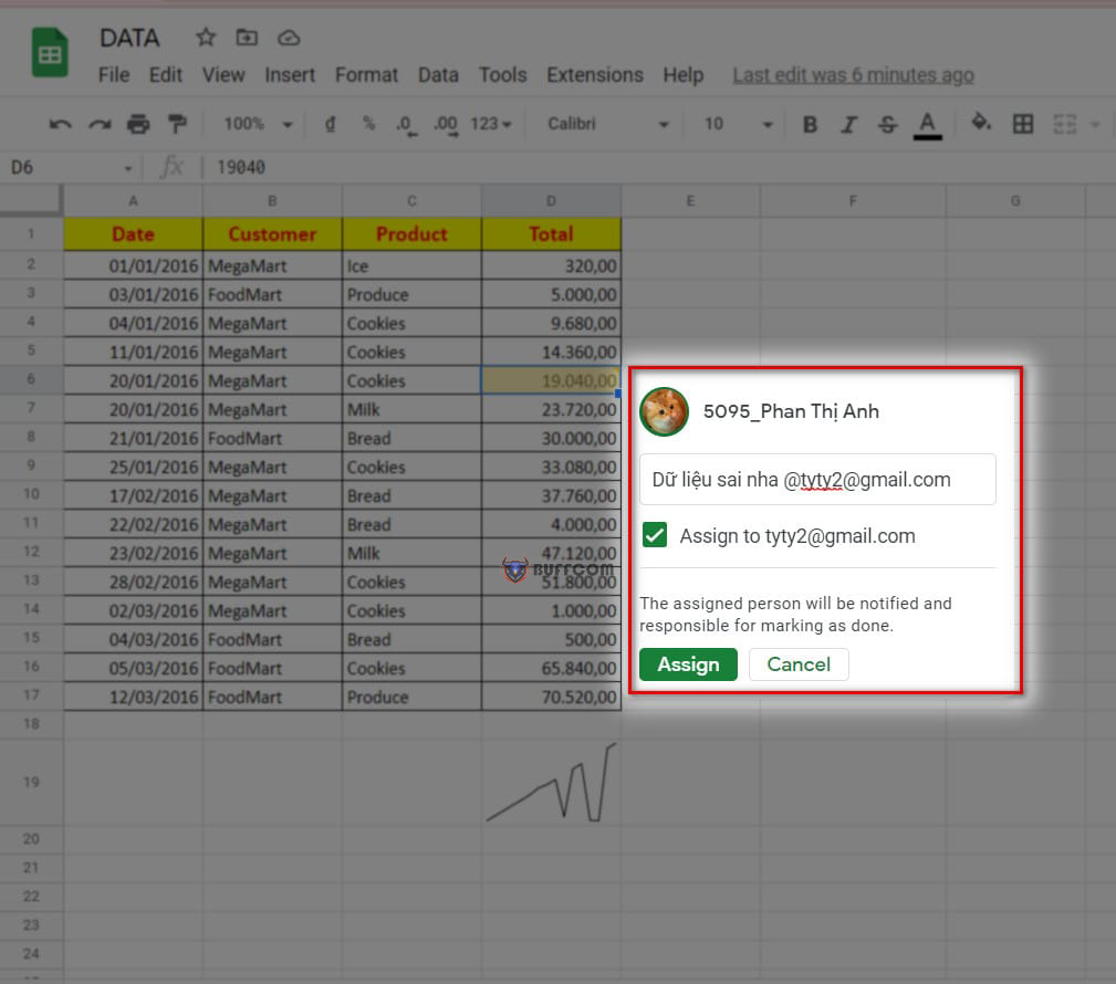
 And people who access the sheet will see your comment and adjust accordingly.
Note: If you want people to see your comment quickly to adjust in time. You can tag everyone’s email in the comment box. By adding “@” after the comment line, you can type the email name of the person you want to send it to.
Tip 3: Verify Email addresses in Google Sheets
During work, you want to send an email to the list of emails entered in the spreadsheet. But you want to check if that Email is correct or exists? A feature that cannot be missed helps you check it out!
First, you select the cell to check the email.
Next, you will type: =ISEMAIL(B3)
Explanation: B3: is the cell containing the email you want to check.
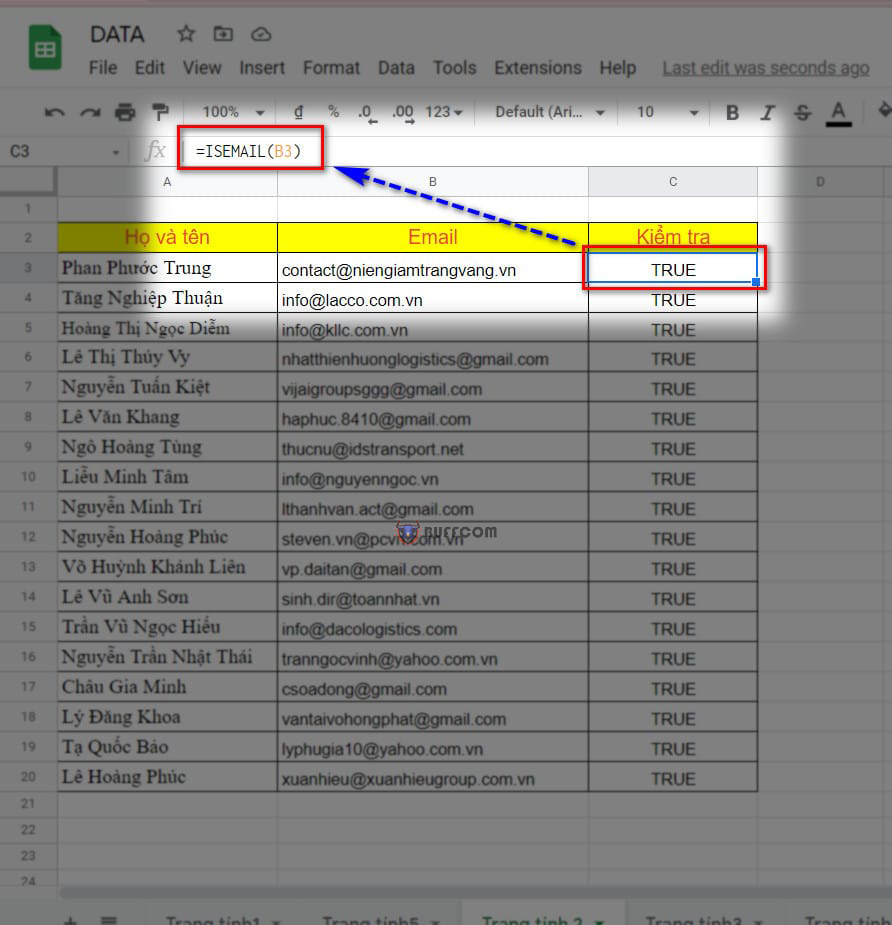 If the result displayed is True, then the email has been entered correctly and you can confidently send it to everyone!
Tip 4. Creating QR codes in Google Sheets
You want to create a QR code for your website. Usually, you would need to download an app or ask someone to do it for you. However, with this 4th tip, you won’t have to go through the trouble or ask anyone for help anymore!
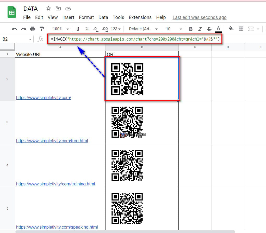
In Google Sheets, there’s a feature that allows you to create QR codes quickly with the following syntax: =IMAGE(“https://chart.googleapis.com/chart?chs=200×200&cht=qr&chl=”&cell containing the website URL&””)
For example, let’s say you want to create a QR code for the website shown in the image below:
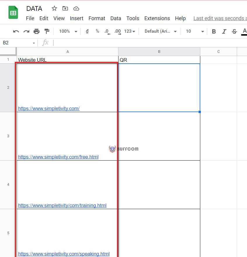 And you want to create QR codes for the other websites as well. Using the syntax above, you would type the following:
=IMAGE(“https://chart.googleapis.com/chart?chs=200×200&cht=qr&chl=”&A2&””)
Explanation: A2 is the cell containing the URL of the website you want to create a QR code for.
 Tip 5. Removing spaces in the name field
When you have a spreadsheet containing a list of employee names in your company, sometimes the names are disorganized and have a lot of unnecessary spaces. You want to process that list, but don’t know how? Don’t worry, Google Sheets has a feature to help you with that!
First, in the cell where you want to display the result after processing, type: =TRIM(A2)
Explanation: A2 is the cell containing the data that needs spaces to be removed.
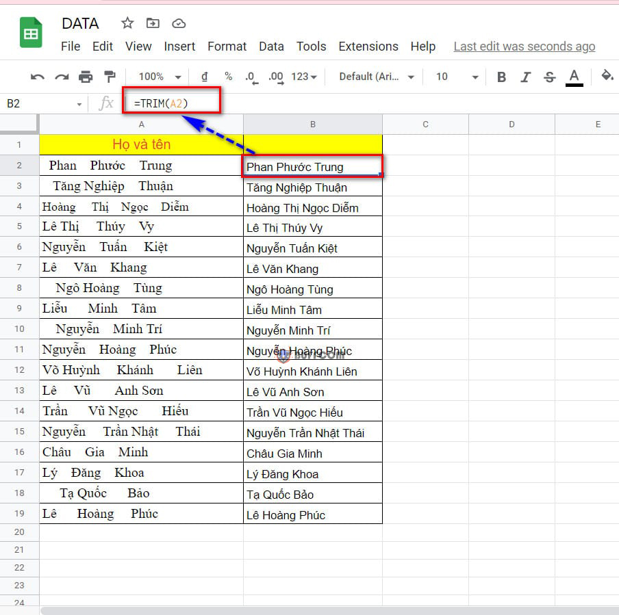
And that’s it! I’ve just taught you 5 tips in Google Sheets that users need to know. I hope this article from Buffcom.net helps you. If you find it useful, don’t forget to rate the article below to help me out! Best regards.

