Understanding everything about IFERROR function in Excel, Google Sheets

In this article, Buffcom.net will explain what IFERROR is and how to use it, which not everyone knows.
IFFERROR is a quite special function, not used much in Excel and Google Sheets. For many of you, you may still not know what IFERROR is, how to use it, and how to combine it with other functions. So, to understand more clearly, let’s refer to the following article with Buffcom.net.

What is the IFERROR function?

The IFERROR function in Excel is designed to trap and manage errors in formulas and calculations. Specifically, IFERROR checks a formula, and if it results in an error, it returns a specified value you choose; otherwise, it returns the formula’s result.
The syntax of the IFERROR function in Excel is as follows:

Value (required) – what to check for errors. It can be a formula, expression, value, or cell reference.
Value_if_error (required) – the value to return if an error is found. It can be an empty string (blank cell), text message, numeric value, another formula, or calculation.

For example, when dividing two columns of numbers, you may encounter a series of different errors if one of the columns contains empty cells, non-numeric or text values.

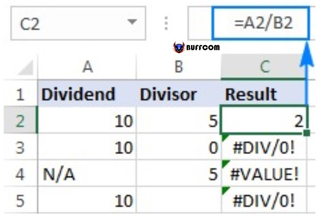To prevent that from happening, use the IFERROR function to trap and handle errors the way you want.
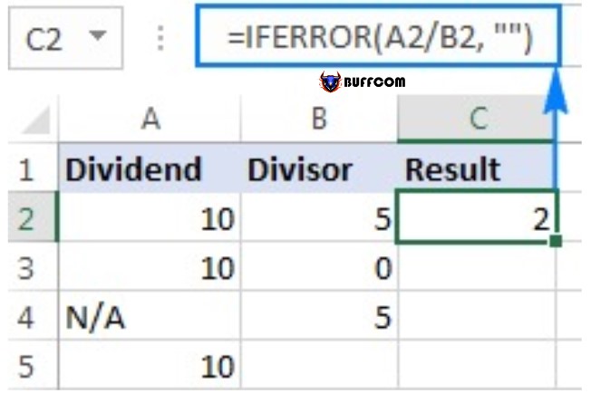
If an error occurs, then leave it blank. Then, provide an empty string (“”) for the value_if_error argument to return a blank cell if an error is found:

=IFERROR(A2/B2, “”)

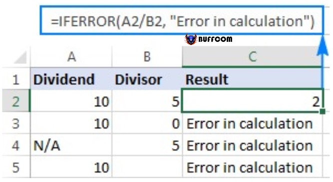
If an error occurs, then you want to display your own message instead of Excel’s standard error sign:

=IFERROR(A2/B2, “Error in calculation”)

5 things you should know about the IFERROR function

The IFERROR function in Excel handles all types of errors including #DIV/0!, #N/A, #NAME?, #NULL!, #NUM!, #REF!, and #VALUE!.
Depending on the content of the value_if_error argument, IFERROR can replace errors with your custom text message, number, date, or logical value, the result of another formula, or an empty string (blank cell).
If the value argument is a blank cell, it is considered an empty string (“”) but not an error.
IFERROR was introduced in Excel 2007 and is available in all subsequent versions of Excel 2010, Excel 2013, and Excel 2016.

Example applications of the IFERROR function

The following examples demonstrate how to use the IFERROR function in Excel and Google Sheets in combination with other functions to accomplish more complex tasks.

IFERROR with VLOOKUP

One of the most common uses of the IFERROR function is to let the user know that the value they are looking for does not exist in the dataset. For this, you place a VLOOKUP formula inside IFERROR like this:

IFERROR(VLOOKUP(…), “Not found”)

If the lookup value is not found in the table you are searching, the regular VLOOKUP formula will return the #N/A error:

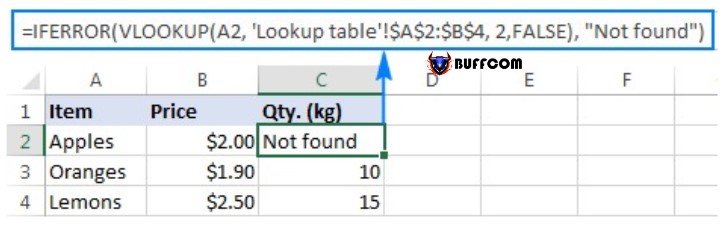
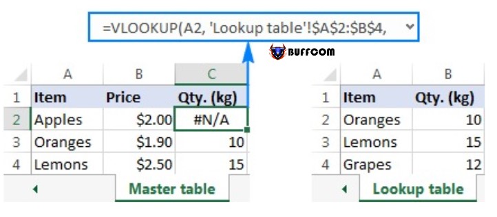For your users, wrap the VLOOKUP formula in IFERROR and display a user-friendly and informative message:
=IFERROR(VLOOKUP(A2, ‘Lookup table’!$A$2:$B$4, 2,FALSE), “Not found”)
The screenshot below shows this IFERROR formula in Excel:

If you only want to trap the #N/A error but not all errors, use the IFNA function instead of IFERROR.

Nested IFERROR functions to perform sequential VLOOKUPs

In situations where you need to perform multiple VLOOKUPs based on the success or failure of a previous VLOOKUP, you can nest two or more IFERROR functions inside another function.
Suppose you have some sales reports from the company’s regional branches and you want to get the amount for a specific order ID. With A2 as the lookup value in the current worksheet and A2:B5 as the lookup range in 3 lookup worksheets (Report 1, Report 2, and Report 3), the formula is as follows:
=IFERROR(VLOOKUP(A2,’Report 1′!A2:B5,2,0),IFERROR(VLOOKUP(A2,’Report 2′!A2:B5,2,0),IFERROR(VLOOKUP(A2,’Report 3′!A2:B5,2,0),”not found”)))
The result will look like this: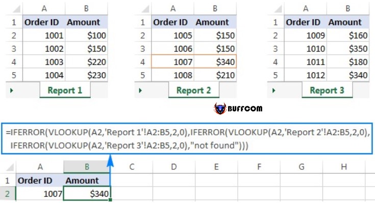

IFERROR in array formulas

As you may know, an array formula in Excel means performing multiple calculations in a single formula. If you provide an array formula or an expression that leads to an array in the value argument of the IFERROR function, it will return an array of values for each cell in the specified range. The following example shows the details.
Suppose you have Total in column B and Price in column C, and you want to calculate Total quantity. This can be done using the following array formula, which divides each cell in the range B2:B4 by its corresponding cell in the range C2:C4, then adds up the results:
=SUM($B$2:$B$4/$C$2:$C$4)
The formula works fine as long as the divisor range does not have any 0s or blank cells. If there is at least one 0 or blank value, the #DIV/0! error value is returned.

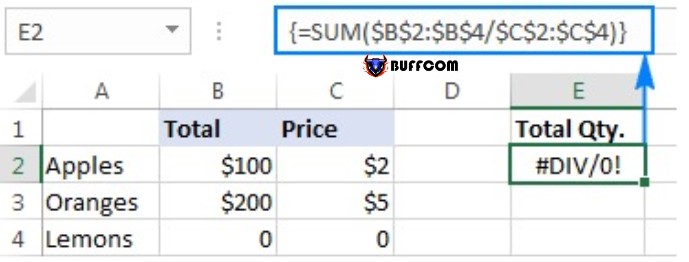To fix this error, simply perform a division operation within the IFERROR function:
=SUM(IFERROR($B$2:$B$4/$C$2:$C$4,0))
The formula divides a value in column B by a value in column C for each row (100/2, 200/5, and 0/0) and returns the result array {50; 40; #DIV/0!}. The IFERROR function catches all #DIV/0! errors and replaces them with zero. Then, the SUM function adds the values in the result array {50; 40; 0} and outputs the final result (50 + 40 = 90).

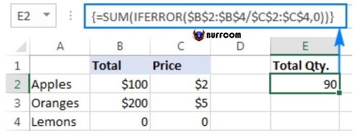Note: Remember that array formulas must be completed by pressing Ctrl + Shift + Enter – a shortcut.

IFERROR vs IF ISERROR

Now that you know how to easily use the IFERROR function in Excel, you may wonder why some people still lean towards using a combination of IFERROR. What are the advantages of using IF ISERROR compared to IFERROR? None. In the old days of Excel 2003 and earlier, when IFERROR did not exist, IF ISERROR was the only way to trap errors. In Excel 2007 and later versions, it’s a bit more complicated to achieve similar results.

For example, to catch VLOOKUP errors, you can use one of the following formulas:
In Excel 2007 – Excel 2016:
IFERROR(VLOOKUP(…), “Not found”)
In all versions of Excel:
IF(ISERROR(VLOOKUP(…)), “Not found”, VLOOKUP(…))

Note that in the VLOOKUP IF ISERROR formula, you have to use VLOOKUP twice. In plain English, the formula can be read as follows: If the VLOOKUP result is an error, return “Not found,” otherwise output the VLOOKUP result.

Here’s a real-life example of the Excel IF ISERROR VLOOKUP formula:
=IF(ISERROR(VLOOKUP(D2, A2:B5,2,FALSE)),”Not found”, VLOOKUP(D2, A2:B5,2,FALSE))

IFERROR vs IFNA

Introduced with Excel 2013, IFNA is another function to check for formula errors. Its syntax is similar to IFERROR:
IFNA(value, value_if_na)
How is IFNA different from IFERROR? – The IFNA function only catches #N/A errors, while the IFERROR function handles all types of errors.
When might you want to use IFNA? – For example, when working with important or sensitive data, you may want to be alerted to potential errors in your data set and have Excel display standard error indicators with a “#” symbol that can be visually striking.

See how you can create a formula to display the “Not found” message instead of the #N/A error, which appears when the lookup value is not found in the data set, but draws your attention to other Excel errors.

Suppose you want to pull Qty. from the lookup table to the summary table as shown in the screenshot below. Using the IFERROR VLOOKUP formula in Excel will create a visually appealing result, but it’s technically inaccurate because Lemons exist in the lookup table:

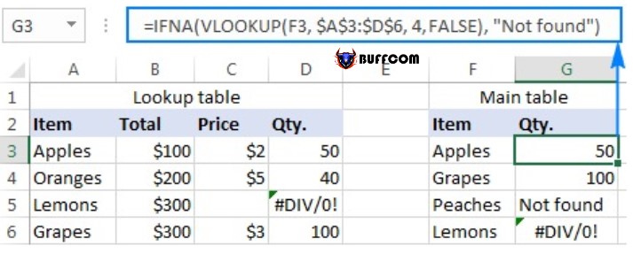
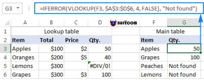To catch #N/A but display #DIV/0 error, use the IFNA function in Excel 2013 and Excel 2016: =IFNA(VLOOKUP(F3,$A$3:$D$6,4,FALSE), “Not found”) Or, combine IF ISNA in Excel 2010 and earlier versions: =IF(ISNA(VLOOKUP(F3,$A$3:$D$6,4,FALSE)),”Not found”, VLOOKUP(F3,$A$3:$D$6,4,FALSE)) The syntax of the IFNA VLOOKUP and IF ISNA VLOOKUP formulas are similar to the previously discussed IFERROR VLOOKUP and IF ISERROR VLOOKUP formulas. As shown in the screenshot below, the Ifna VLOOKUP formula only returns “Not found” for the item not found in the lookup table (Peaches). For Lemons, it displays #DIV/0! indicating that our lookup table contains a divide by zero error:

Best practices for using the IFERROR function

Now that you know that the IFERROR function is the easiest way to catch errors in Excel and conceal them with blank cells, 0 values, or your custom messages. However, that doesn’t mean you should end each formula with error handling. The simple suggestions below can help you strike a balance. Don’t make errors for no reason. Use the smallest possible package of a formula in IFERROR. To only handle specific errors, use the error handling function with a smaller scope:

• IFNA or IF ISNA to only catch #N/A errors.
• ISERR to catch all errors except #N/A errors.

Above, Buffcom.net has explained what IFERROR is. If you have any further questions, please comment below. Don’t forget to Like and Share if you find this article helpful, as it will motivate Buffcom.net to bring more valuable content in the future.