Using VLOOKUP Nested in VLOOKUP Function in Excel
Using VLOOKUP Nested in VLOOKUP Function in Excel: Sometimes your main table and lookup table do not have a common column, which makes it impossible to perform a regular VLOOKUP. However, there might be a third table that doesn’t contain the information you’re looking for but has a common column with both the main and lookup tables. In this case, you need to use a VLOOKUP nested in another VLOOKUP function to reference and retrieve data from the correct column. This article will share with you the detailed steps on how to do this.
1. VLOOKUP Function Syntax
The syntax of the VLOOKUP function is as follows: =VLOOKUP(Lookup_value, Table_array, Col_index_ num, Range_lookup)
Where:
- Lookup_value: The value you want to search for.
- Table_array: The table range to search for the value, and you need to use F4 to lock the value for the purpose of automatic formula copying.
- Col_index_num: The column number of the data to retrieve in the table being searched.
- Range_lookup: A logical value (TRUE=1, FALSE=0) that determines whether to search for an approximate or exact match in the table range.
Note: - If Range_lookup = 1 (TRUE): Search for an approximate match.
- If Range_lookup = 0 (FALSE): Search for an exact match.
- If this argument is omitted, Excel assumes that Range_lookup = 1.
2. How to Use VLOOKUP Nested in VLOOKUP Function
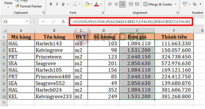
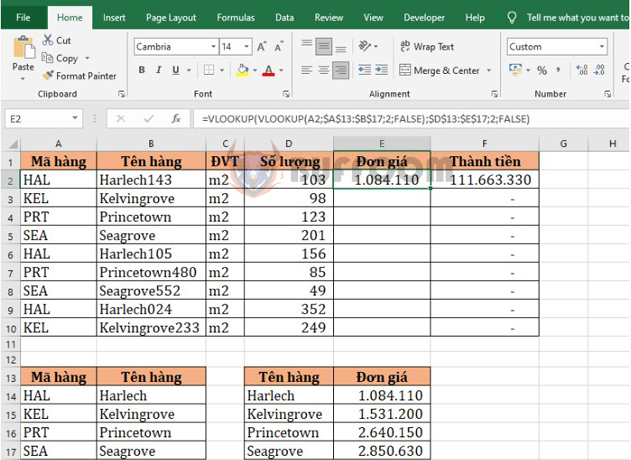
For example, suppose we have three data tables as shown in the figure below. The requirement is to fill in the unit price of each item in the table. We can see that we first need to use the VLOOKUP function to reference the item code to the item name in the second table. Then, we nest another VLOOKUP function to reference the item name to the unit price in the third table.
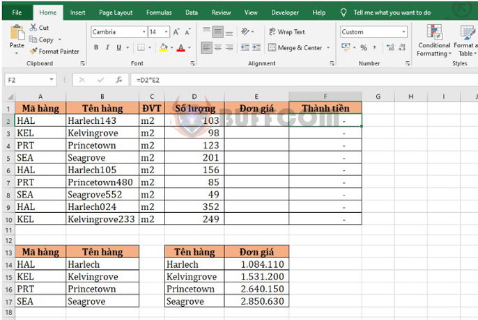
Specifically, we will have the formula to find the unit price in cell E2 as follows:
Using VLOOKUP Nested in VLOOKUP Function in Excel
=VLOOKUP(VLOOKUP(A2;$A$13:$B$17;2;FALSE);$D$13:$E$17;2;FALSE)
The above function means that we first use the item code HAL in cell A2 to reference the item name in table 2, which gives us the result Harlech. Next, we use the item name Harlech that we just referenced to reference the unit price in table 3, which gives us the result of 1,084,110.
Using VLOOKUP Nested in VLOOKUP Function in Excel
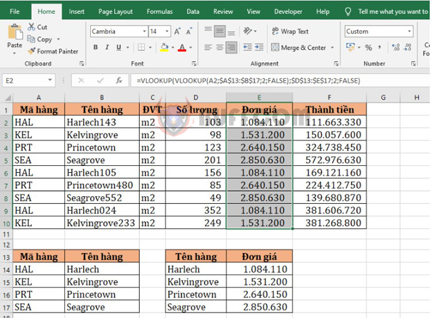
Note that you need to press F4 to lock the reference to the data tables so that you can copy the formula to other cells. Next, copy the formula to other cells in the table, and you will find the unit price for all items in the table.
Using VLOOKUP Nested in VLOOKUP Function in Excel
In summary, Excel is a powerful tool that offers many functions to help users manage and analyze their data effectively. Among these functions, VLOOKUP is one of the most commonly used ones, allowing users to search for specific data in a table and retrieve corresponding values based on a given search key. By mastering the techniques and tips shared in this article, you can improve your proficiency in using VLOOKUP and enhance your productivity in working with Excel. Whether you are a student, a professional, or a data enthusiast, Excel and VLOOKUP can be valuable assets to your skill set. So keep practicing and exploring, and you may discover even more useful features of Excel that can benefit your work and life.

