5 Excel Tips and Hacks
5 Excel Tips and Hacks. In this article, I will show you 5 tips and hacks for MS Excel. These tips will help you become an Excel genius! Let’s explore the article below.
1. Encode formulas using the F9 function
5 Excel Tips and Hacks
With this tip, you can view all the formulas in a calculation.
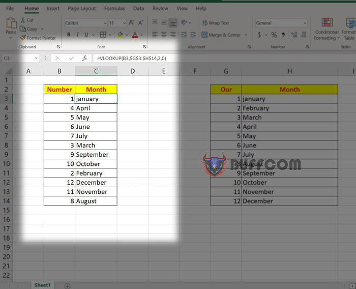
To understand better, let’s take an example:
In the above example, I have a formula =VLOOKUP(B3,$G$3:$H$14,2,0). And you want to display the details of the values in the data range in the formula with the following steps:
First, at the formula, you highlight the data range: $G$3:$H$14.
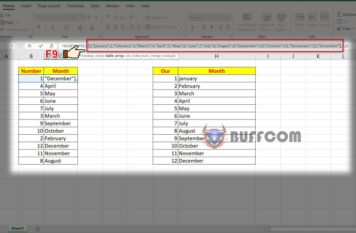
Next, press the F9 key combination. Automatically, the data range will show the specific values within the selected range.
5 Excel Tips and Hacks
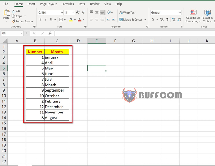
And when you delete the original data range, the results of the returned values will not be lost or incorrect.
5 Excel Tips and Hacks
2. View multiple Excel worksheets in one interface
5 Excel Tips and Hacks
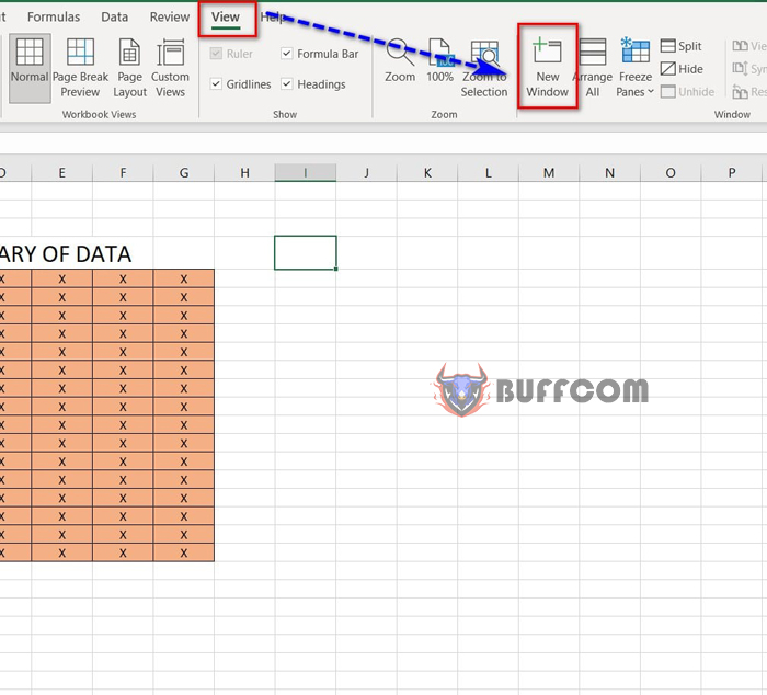
While working, you want to view multiple worksheets at the same time to conveniently type, copy, or compare 2 or more different worksheets. To do this, you will do the following:
First, go to the View tab => New Windows.
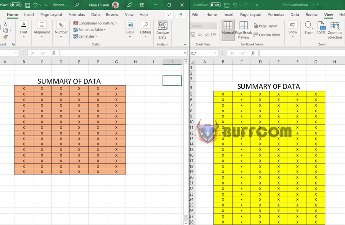
The screen is divided into multiple windows containing multiple Excel files to help you perform tasks easily.
5 Excel Tips and Hacks
3. Fill in data in blank cells
5 Excel Tips and Hacks
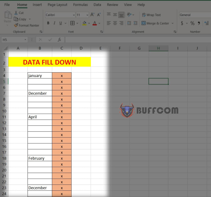
For example, I have a data table like this:
As you can see in the above data, in the first column, I have many blank positions. And you need to add the values of the cells above to each of these blank cells to make the data specific, complete, and more beautiful. With the following method:
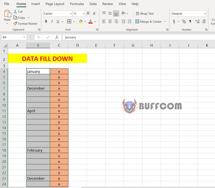
First, you highlight the data range in column 1.
5 Excel Tips and Hacks
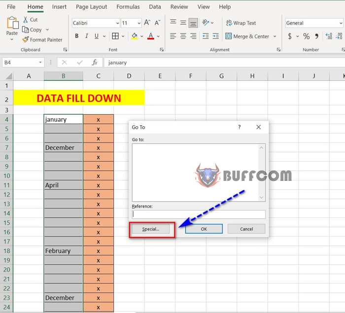
Next, press CTRL + G to open the Go To dialog box and select the Special item.
5 Excel Tips and Hacks
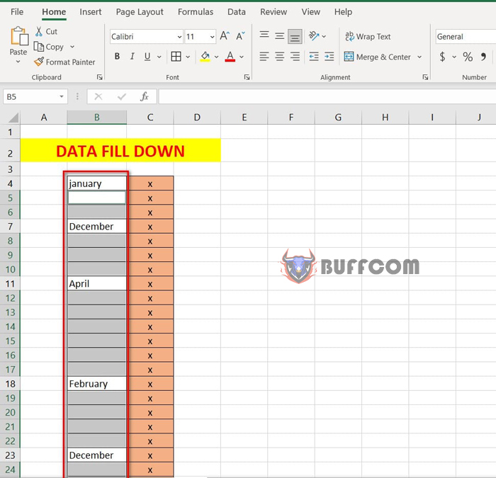
Display the Go to Special table, select Blanks, and click OK. Automatically, the blank cells in the data range are highlighted.
5 Excel Tips and Hacks
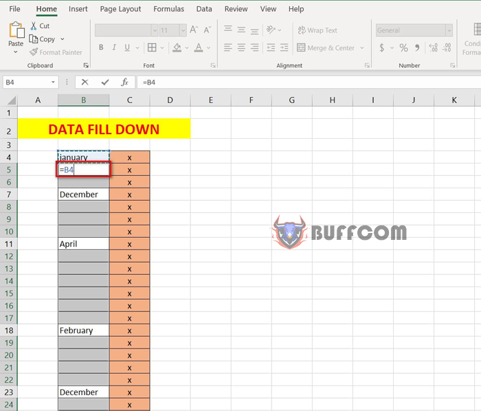
Next, at the first cell, you type “=” + up arrow on the keyboard to select the value in the previous cell.
5 Excel Tips and Hacks
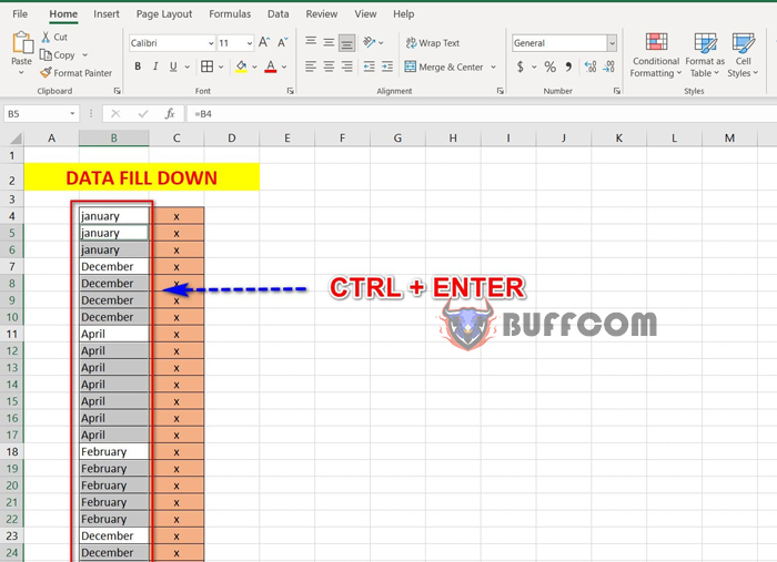
And press CTRL + ENTER to display the result.
5 Excel Tips and Hacks
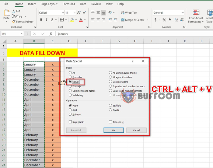
Next, you highlight the range of displayed results and press CTRL + ALT + ENTER to open the Paste Special dialog box.
In the dialog box, select Values and click Ok to display the result in the form of values instead of relying on formulas.
5 Excel Tips and Hacks
4. Creating a dropdown list
To create a dropdown list from a data range, follow these steps:
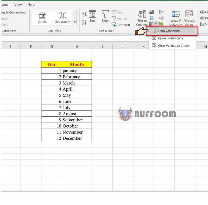
Step 1: Select the cell where you want to display the dropdown list, go to the Data tab => Data Validation.
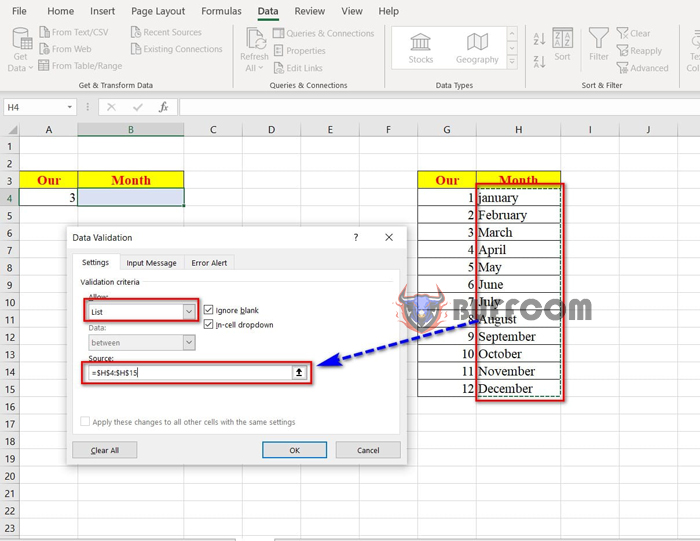
 Step 2: In the Data Validation dialog box, select “List” from the “Allow” dropdown, and then select the data range that contains the list you want to use for the dropdown in the “Source” field.
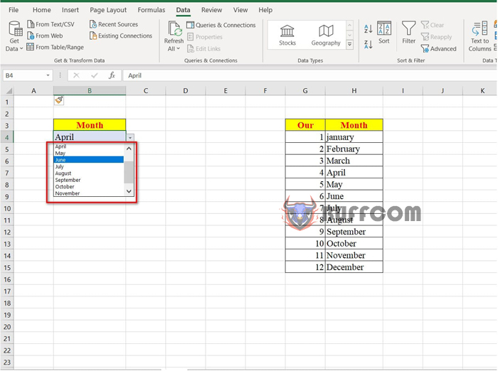
 Step 3: Click OK to complete the process.
 5. Locking/Protecting formula cells
When working with important data, you may want to lock the cells containing formulas to prevent others from changing them. To do this, follow these steps:
First, select all the cells in Excel and press CTRL + 1.
In the Format Cells dialog box, select the “Protection” tab, and uncheck the “Locked” option.
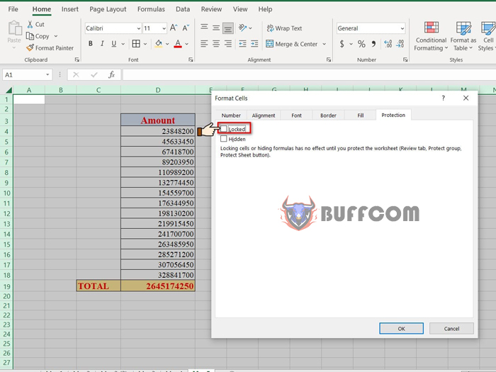 Next, select the cell containing the formula you want to lock, and press CTRL + 1.
In the Format Cells dialog box, select the “Protection” tab, and check the “Locked” option.
 Click OK to complete the process.
One more step is to go to the Review tab => Protect Sheet. In the Protect Sheet dialog box, check both “Select locked cells” and “Select unlocked cells” options.
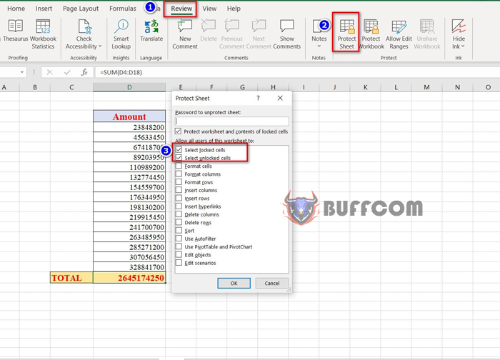 Click OK to complete the process.
Now, when others access the Excel file and try to select any formula cell, they will not be able to select it.
That’s it! I hope these 5 tricks in MS Excel will be helpful for you. If you found this article helpful, don’t forget to rate it below. Thank you!


