3 Small Excel Tricks You Need to Know

3 Small Excel Tricks You Need to Know, Excel is a versatile and widely used tool today. In Excel, you can perform calculations, create plans, draw charts, and more, but knowing additional tricks in Excel will make your use of the tool more efficient. Today, I will guide you through 3 small tricks in Excel that you need to know.
3 Small Excel Tricks You Need to Know Sparklines Chart
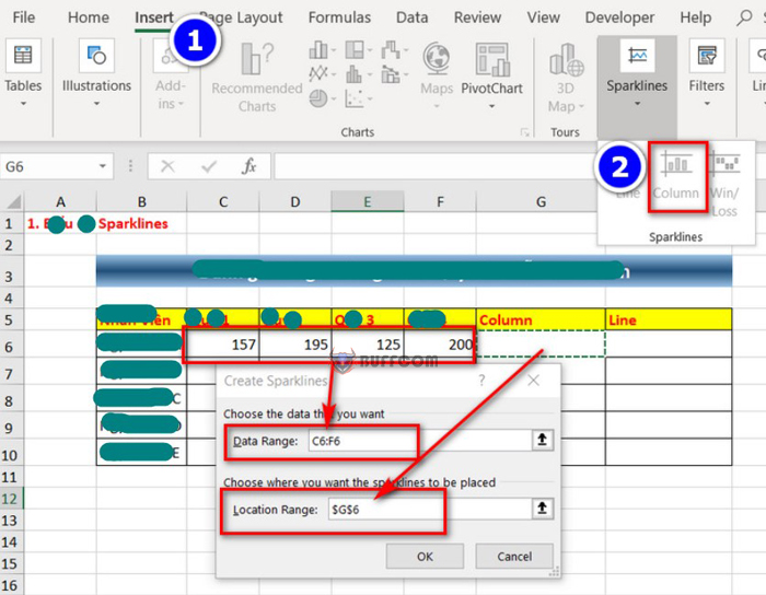
Suppose you have a list of employees and you want to create a chart to evaluate their competency by quarter. To start creating a chart to evaluate employees’ competency, you go to Insert -> in Sparklines, there are two types of charts that can show the development trend of that employee: Column and Line.
With the Column chart, the information for each quarter of the employee will be represented by a column, which is quite easy for observation. Choose Column and in the new window, in the Data Range box, select the employee’s quarterly data and in the Location Range box, click on where you want this chart to appear.
3 Small Excel Tricks You Need to Know
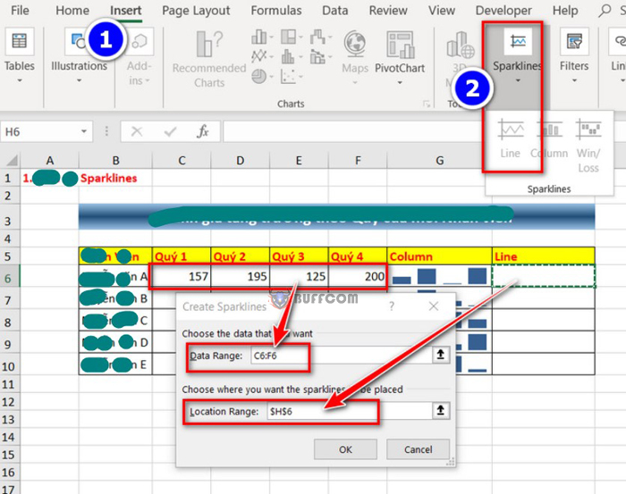
With the Line chart, you perform the same steps as the Column chart, but the Line chart shows the quarters as points on the chart, and these points are connected by lines, so this chart is called a Line chart.
3 Small Excel Tricks You Need to Know
Deleting Blank Rows
In a list of employees or a sales report that contains blank rows, these empty rows will reduce the aesthetic value of the report and, of course, be evaluated poorly. To solve this problem, you can also delete blank rows, but if you have a list of hundreds of rows and many of them are empty, sitting down to filter and delete them will take a lot of time and effort. Now I will guide you on how to delete blank rows without having to sit down to filter and delete.
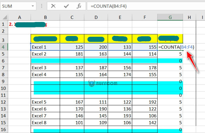
First, you will use the COUNTA function to automatically check for blank rows by clicking on the cell after the first row, typing =COUNTA(select the data range of that row) -> Enter. This function will return the number of cells that have data in that row. Now click on the lower right corner of this cell and drag it down to the last row of the data. If a row has data, it will return a number, and if a row does not have data, it will return 0.
Note: If your data is large, you can copy the cell just created with the COUNTA function and drag it down to the end of the data range, click on the bottom cell of the range with the last row, press Shift+Up arrow to highlight this area, and Ctrl+V to paste it.
3 Small Excel Tricks You Need to Know
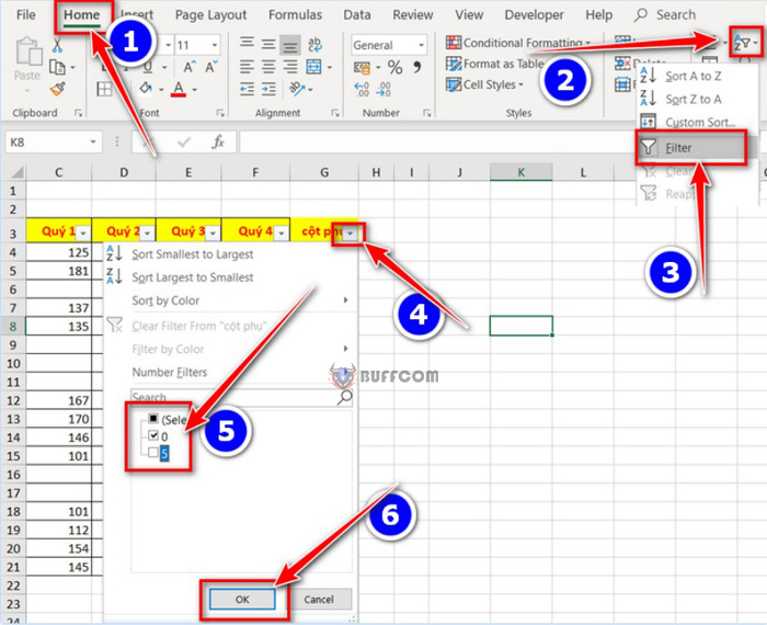
Next, go to Home -> Sort & Filter -> Filter. Now, on the columns with filters, select the filter of the secondary column, remove the checkmark of number 5, and leave a checkmark on number 0 -> ok.
3 Small Excel Tricks You Need to Know
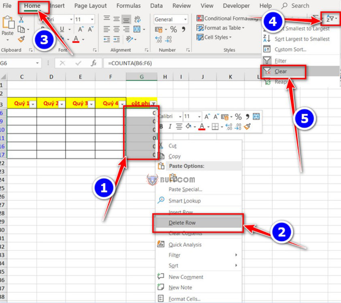
Now, only show the row with 0 by selecting the secondary column of all rows with 0 -> right-click and select Delete Row -> ok. Now you have deleted the rows with 0, go to Home -> Sort&Filter -> Clear.
3 Small Excel Tricks You Need to Know
Therefore, your list is now perfect and there are no more blank rows in the middle of the list.
Creating diagonal lines in cells
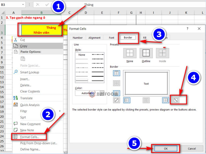
Sometimes, you may want to create diagonal lines in cells to visually separate information in the cell. To create diagonal lines in a cell, click on the cell you want to add lines to, then go to Home -> Borders -> More Borders. In the new window, click on the diagonal line icon, select the diagonal line style you want to add, and click ok.
3 Small Excel Tricks You Need to Know
These are 3 small tricks in Excel that can be useful for your daily work.


