Tips for quickly comparing data tables in Excel
Tips for quickly comparing data tables in Excel: During the process of working with Excel, comparing and matching data is a common task, especially for accountants. In this article, Buffcom.net will share with you how to compare data tables in Excel.
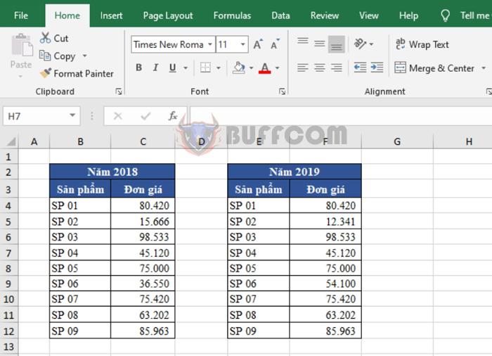
For example, let’s say we have two tables of prices for products from 1 to 9 in the years 2018 and 2019 as shown in the figure below. The requirement is to compare which product prices in 2019 have changed compared to 2018, and which product prices in 2019 remain the same as in 2018. To compare, please follow the steps below.
Step 1
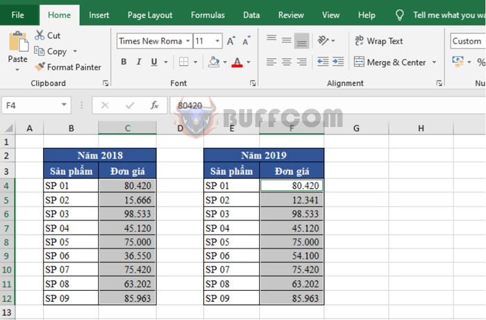
To compare prices between two years, first select and highlight all the data that needs to be compared in the two tables. Drag the mouse to select the 2018 data table. Then press and hold Ctrl and drag the mouse to select the 2019 data table.
Tips for quickly comparing data tables in Excel
Step 2
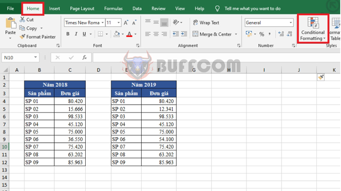
Next, select the Home tab on the toolbar. Then select Conditional Formatting under the Styles section.
Tips for quickly comparing data tables in Excel
Step 3
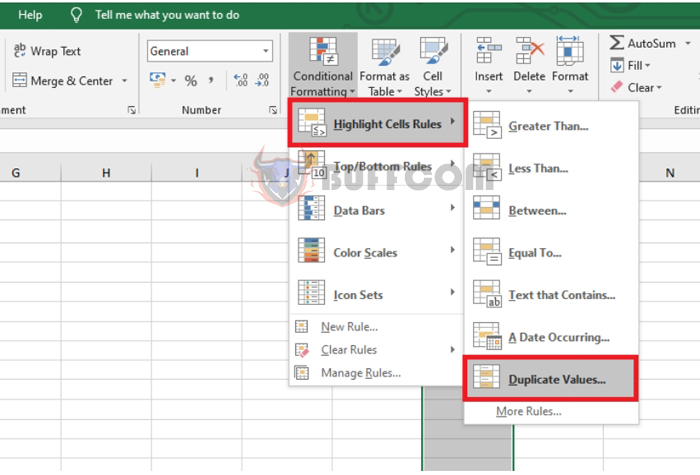
The scroll bar appears, select Highlight Cells Rules. Next, select Duplicate Values.
Tips for quickly comparing data tables in Excel
Step 4
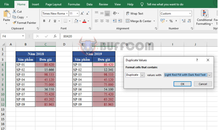
At this point, the Duplicate Values dialog box appears. Under the Format cells that contain section, select Duplicate to highlight cells with duplicate data. Under the Values with section, you can click to select a color, highlight border. Here are the colors for you to choose from:
- Light Red Fill with Dark Red Text: Highlight cells with light red background and dark red text
- Yellow Fill with Dark Yellow Text: Highlight cells with yellow background and dark yellow text
- Green Fill with Dark Green Text: Highlight cells with green background and dark green text
- Light Red Fill: Highlight cells with light red background
- Red Text: Highlight cells with red text
- Red Border: Highlight cells with red border
- Custom Format: Select custom colors as desired
After you have made your selection, click OK to complete. You can see that the products whose prices in 2019 have not changed compared to 2018 have been highlighted, namely SP 01, 03, 04, 05, 07, 08, 09.
Tips for quickly comparing data tables in Excel
Step 5
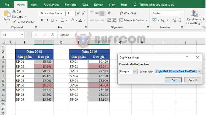
If you want to highlight the data that does not match, simply select Unique under the Format cells that contain section. Then click OK to complete. You can see that the products whose prices in 2019 have changed compared to 2018 have been highlighted, namely SP 02 and SP 06.
Tips for quickly comparing data tables in Excel
So, this article has guided you on how to compare data tables in Excel. Hopefully, this article will be useful to you in your work. Wish you success!


