How to Use Slicer Tool to Filter Data in Excel
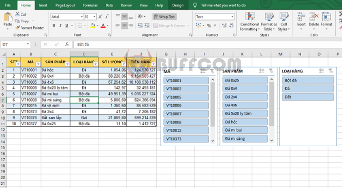
How to Use Slicer Tool to Filter Data in Excel: Slicer is a highly useful tool in Excel that allows users to filter data. Follow the steps below to learn how to use the Slicer tool in Excel.
To use the Slicer tool, first you need to create a Slicer for your table by following these steps:
Step 1
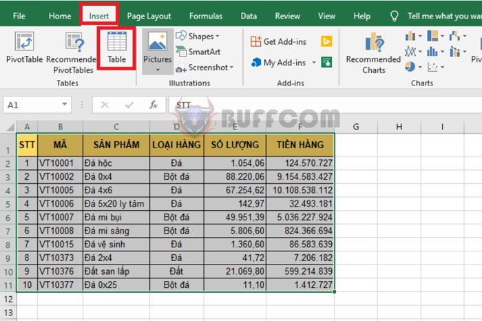
Before creating a Slicer, you need to create a table for your data. Highlight the data range that needs to be filtered. Then, select the Insert tab on the ribbon. Next, click on the Table icon to format the table for the data.
How to Use Slicer Tool to Filter Data in Excel
Step 2
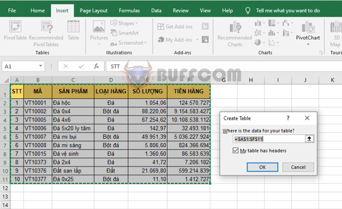
Now, the Create Table dialog box will appear. Select the data range for the table in the “Where is the data for your table” section. Check the box for “My table has headers“. Finally, click OK to complete.
How to Use Slicer Tool to Filter Data in Excel
Step 3
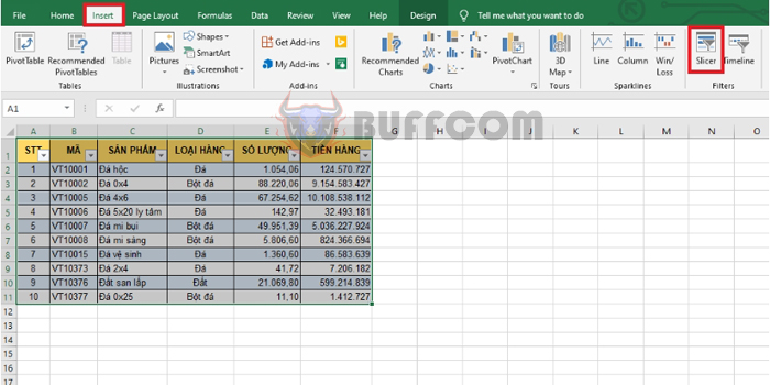
After the data is formatted as a table, highlight the entire table and select the Insert tab on the ribbon. Next, click on the Slicer icon in the Filters section.
How to Use Slicer Tool to Filter Data in Excel
Step 4
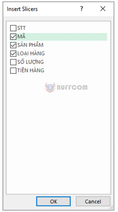
Now, the Insert Slicers dialog box will appear. Check the boxes for the columns that need to be filtered. In this case, we need to filter the columns: Code, Product, and Product Type. Therefore, we will select these columns. Finally, click OK to complete.
How to Use Slicer Tool to Filter Data in Excel
Step 5
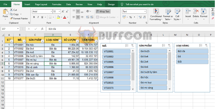
The results will show the Slicers of the selected columns. Simply click on the items to filter the data in the table as desired.
How to Use Slicer Tool to Filter Data in Excel
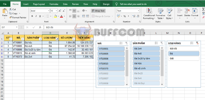
For example, to filter the product type to “stone”, simply click on the “stone” item in the Product Type table. This will filter all stone products. We can see that the stone products include: Stone 2×4, Stone 4×6, Stone 5×20 centrifuge, Stone hob, and Stone toilet in the Product table.
How to Use Slicer Tool to Filter Data in Excel
In this way, this article has provided you with the steps to use the Slicer tool to filter data in Excel. We hope this article will be useful to you in your work. Good luck!


