How to use the RATE function to calculate the interest rate of a loan in Excel

In this article, Buffcom.net will guide you on how to use the RATE function to calculate the interest rate of a loan in Excel.
1. Syntax of the RATE function
The syntax of the function is as follows: =RATE(nper, pmt, pv, [fv], [type], [guess])
Where:
- Nper: Required argument, which is the loan term.
- Pmt: Required argument, which is the payment made each period.
- Pv: Required argument, which is the loan amount.
- Fv: Optional argument, which is the cash balance you want to have after the final payment is made.
- Type: Optional argument, which is either 0 or 1, indicating when payments are due.
- Guess: Optional argument, which is your estimate of the interest rate.
Note:
- The pmt argument includes both principal and interest payments made each period.
- If pmt is omitted, you must enter the fv argument. If fv is omitted, it is assumed to be 0.
- If type is 0 or omitted, payments are due at the end of each period.
- If type is 1, payments are due at the beginning of each period.
- If guess is omitted, it is assumed to be 10 percent.
2. How to use the RATE function
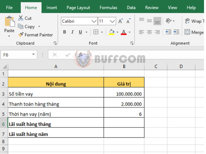
For example, if you borrow 100 million VND from a bank, and you have to repay 2 million VND (including both principal and interest) per month for 6 years, you need to calculate the interest rate of the loan.
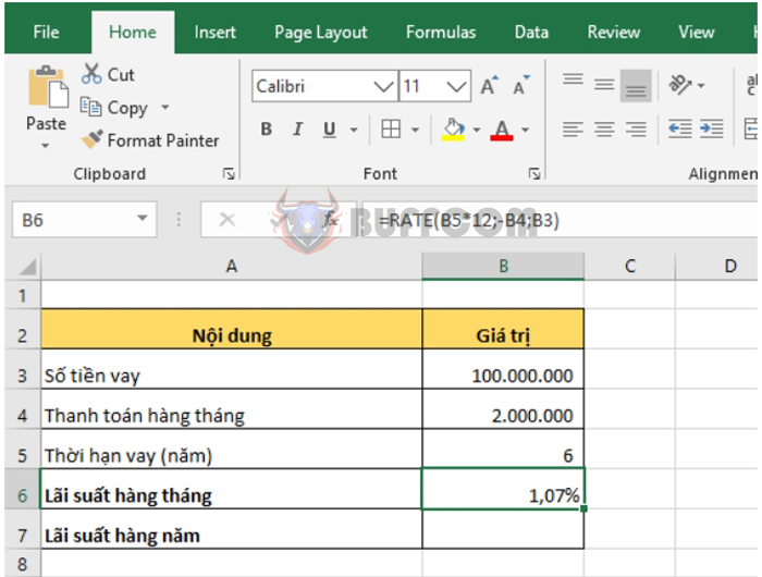
 Using the syntax of the function as described above, we can calculate the monthly interest rate as follows:
=RATE(B5*12,-B4,B3)
We need to multiply B5 by 12 because the loan term is in years and the payment amount is monthly.
 To calculate the annual interest rate, we can simply multiply the monthly interest rate by 12. Alternatively, we can use the following formula:
=RATE(B5,-B4*12,B3)
 Thus, this article has guided you on how to use the RATE function to calculate the interest rate of a loan in Excel. We hope this article will be helpful to you in your work. Good luck!


