How to use the AMORLINC function to calculate depreciation in Excel

How to use the AMORLINC function to calculate depreciation in Excel: Excel provides users with many functions to calculate asset depreciation using different methods. In this article, Buffcom.net will introduce how to use the AMORLINC function to return depreciation for each accounting period by using the depreciation rate. Specific examples in the article will help you easily imagine and quickly learn how to use this function.
1. AMORLINC function structure
Function syntax: =AMORLINC(cost; date_purchased; first_period; salvage; period; rate; [basis])
Where:
Cost: required argument, is the cost of the asset. Date_purchased: required argument, is the date the asset was purchased. First_period: required argument, is the end date of the first period. Salvage: required argument, is the salvage value of the asset. Period: required argument, is the number of depreciation periods. Rate: required argument, is the depreciation rate. Basis: optional argument, is the year basis used.
- Basis = 0 or omitted: One month has 30 days/One year has 360 days (according to the North American standard).
- Basis = 1: The actual number of days in each month/The actual number of days in each year.
- Basis = 2: The actual number of days in each month/One year has 360 days.
- Basis = 3: The actual number of days in each month/One year has 365 days.
- Basis = 4: One month has 30 days/One year has 360 days (according to the European standard).
2. How to use the AMORLINC function
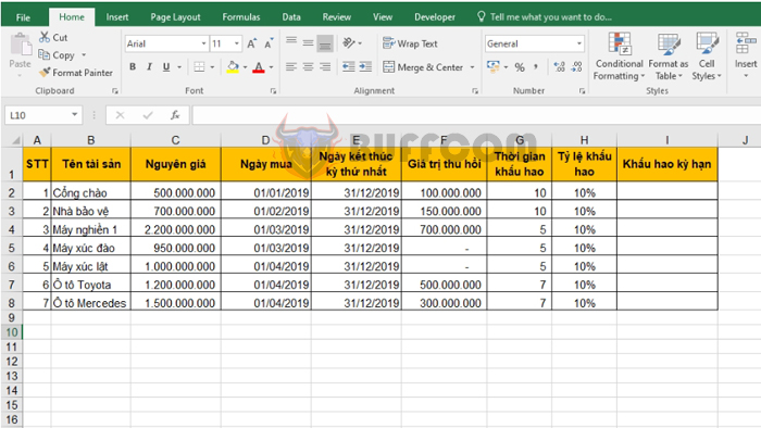
For example, we have a fixed asset depreciation table as shown below. We need to calculate the depreciation for each asset using the AMORLINC function.
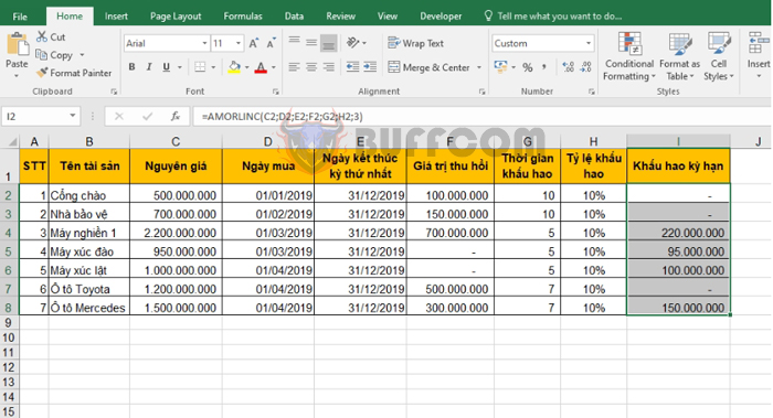
Applying the formula above, we have the depreciation formula for the Gate as follows:

How to use the AMORLINC function to calculate depreciation in Excel
=AMORLINC(C2;D2;E2;F2;G2;H2;3)
Copying the formula for the remaining assets, we obtain the results:

How to use the AMORLINC function to calculate depreciation in Excel
Thus, the above article has instructed you how to use the AMORLINC function to calculate asset depreciation in Excel. Good luck!


