How to quickly hide show Rows or Columns in Excel
How to quickly hide show Rows or Columns in Excel: Sometimes you may want to hide rows or columns that you don’t want to display on the printed version of an Excel worksheet. Or, after printing, you may want to show the hidden rows or columns again. The Hide and Group functions in Excel can help you easily accomplish this.
1. Using Hide to hide/show rows or columns in Excel
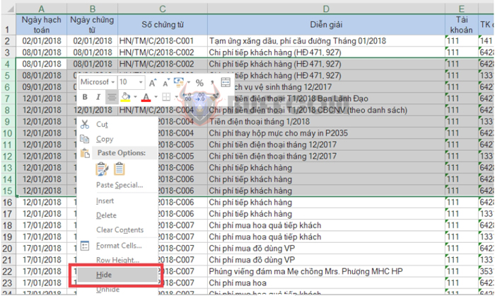
First, select the rows or columns you want to hide. Then, right-click on one of the selected rows or columns and choose Hide.
How to quickly hide show Rows or Columns in Excel
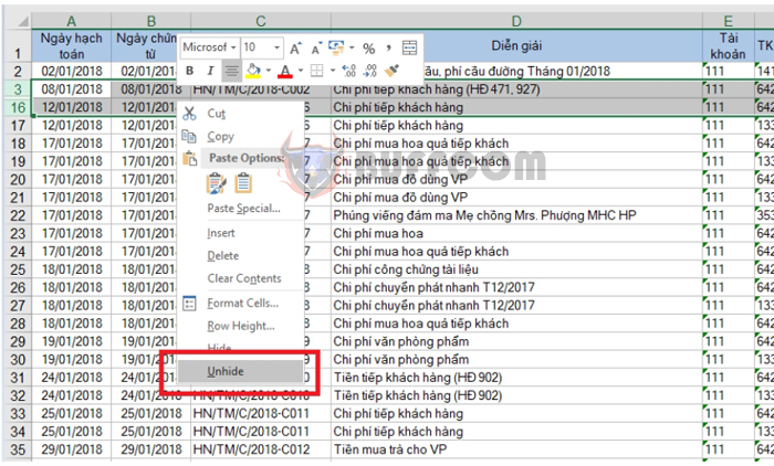
The selected rows or columns will now be hidden. To show them again, you need to select the rows or columns before and after the hidden ones. Then, right-click and choose Unhide.
 2. Using Group to hide/show rows or columns in Excel
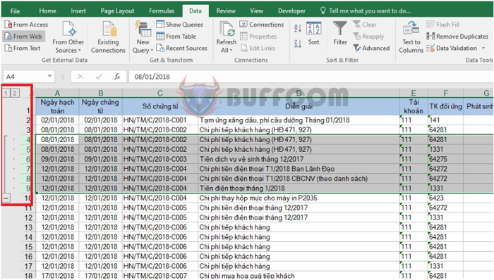
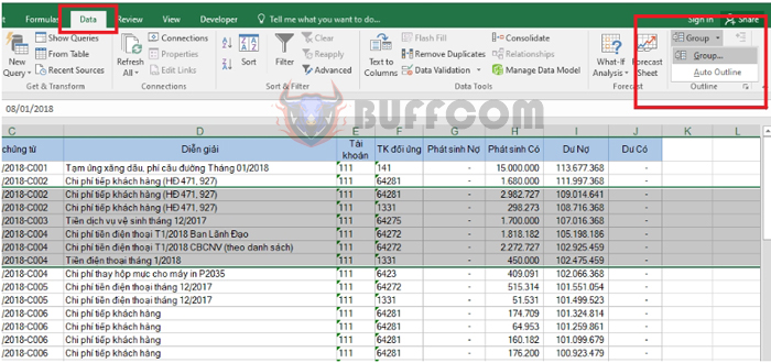
First, select the rows or columns you want to hide. Then, go to the Data tab => in the Outline section, choose Group => Group.
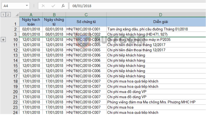
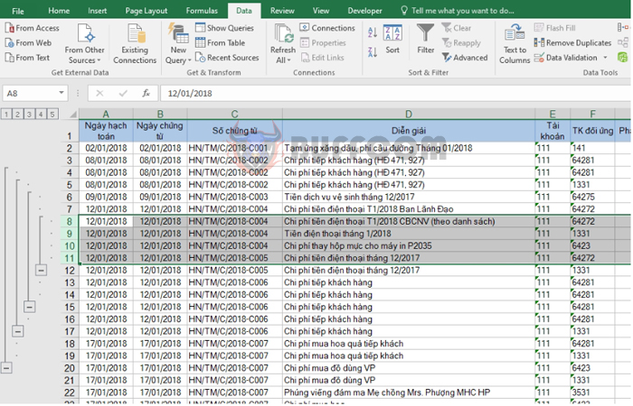
Now, the level 1 and 2 hierarchy will appear on the left side of the screen if you selected rows or above if you selected columns.
 If you want to hide the rows or columns, click on the minus sign (-) => the minus sign will change to a plus sign (+) and the rows will be hidden.
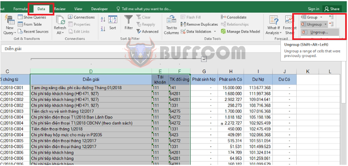
 If you want to remove the Group feature for rows or columns, simply select the rows or columns that have been grouped and hidden => go to the Data tab => Outline => UnGroup => UnGroup.
 3. Creating hierarchical levels for rows or columns
With the Group feature to hide/show rows or columns, you can use this feature to create hierarchical levels for rows and columns, similar to a table of contents in Word.
First, create the level 1 as usual. Then, select the rows you want to create a lower-level group for and proceed as usual. Now, smaller group levels will be created.
 That’s it! This article has introduced you to the methods to hide/show rows and columns in Excel. Good luck!

