How to Wrap Text in Excel 3 Methods

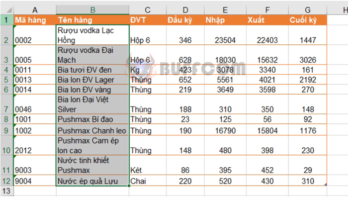
How to Wrap Text in Excel 3 Methods:When working with Excel, if the data in a cell is longer than the cell width, it may overflow into adjacent cells. In such cases, you need to wrap text to display the data in multiple lines for better visibility. This article will guide you through three methods to wrap text in Excel.

1. Wrapping text within a cell

Using the Alt + Enter keyboard shortcut, you can break the text within a cell at any desired position. First, select the cell where you want to wrap the text. Then, place the cursor at the position where you want to break the text.

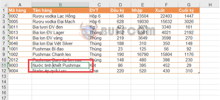Next, press Alt + Enter to insert a line break. The content after the cursor will immediately wrap to the next line.

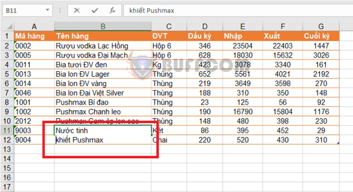2. Using the Wrap Text feature

The Wrap Text feature automatically wraps the text within cells. The line break position depends on the length of the data and the cell width. First, select the cells you want to wrap.

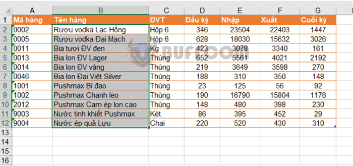
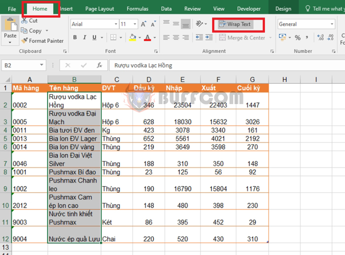
In the Home tab, click on Wrap Text in the Alignment section. The selected cells will automatically wrap the text if the data is longer than the cell width.

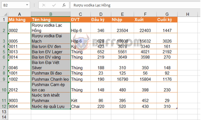
To improve the appearance of the wrapped text, you may need to adjust the cell width accordingly.

3. Customizing the Wrap Text feature in Format Cells

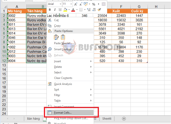
First, select the cell(s) where you want to wrap the text. Then, right-click and choose Format Cells…

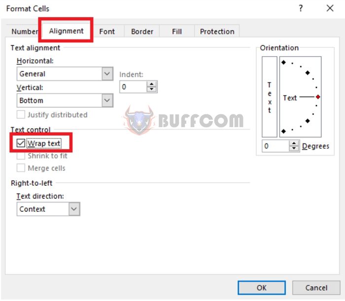
In the Format Cells dialog box, select the Alignment tab. To wrap text within the cell, check the Wrap text option. You can also customize the cell alignment using other available features in the Format Cells dialog box.

The selected cell(s) will now wrap the text and display according to the applied formatting.

How to Wrap Text in Excel 3 Methods

This article has guided you through various methods to wrap text in Excel. Good luck with your Excel tasks!