How to use the DATE function in Excel

How to use the DATE function in Excel. The DATE function in Excel is used to return the numerical value of a date. To convert the output to date format, you can use the Format cell option. In this article, we will learn how to use the DATE function in Excel.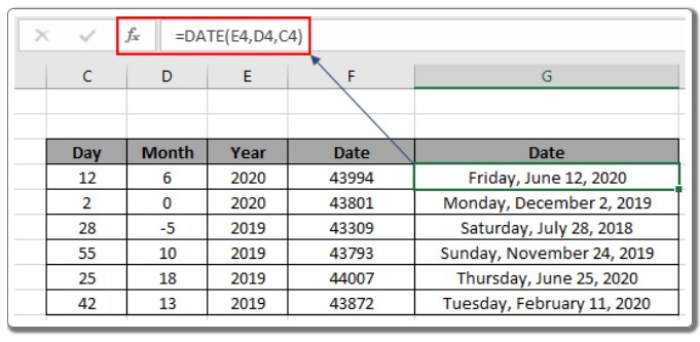

How to use the DATE function in Excel

Syntax of the DATE Function: =DATE(year, month, day)

year: a valid numerical value for the year month: a numerical value for the month, which can be zero or negative day: a numerical value for the day, which can be zero or negative

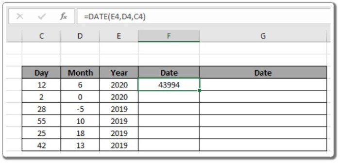
Example of DATE Function: All of these concepts might be confusing to understand. So, let’s test this formula using an example. Here, I have a table with some data. The first column contains numeric values for the day, the second column contains the month value, and the third column contains the year value for the actual date result.

Use the formula: =DATE(E4, D4, C4)

How to use the DATE function in Excel

It will return 43994. In this example, all the arguments for the DATE function are given using cell references. As you can see, the value is not in date format. To change that, simply change the format of the result cell to the desired short or long date format.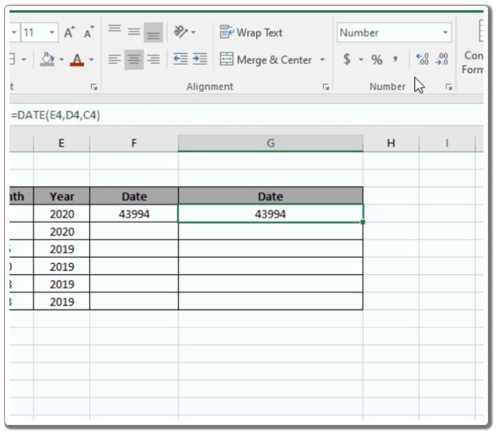

As shown in the animation above, you can change the format of any cell to any format using the Format Cell option. Now you can copy the formula from one cell to the remaining cells using the Ctrl + D shortcut key or the drag-down option in Excel.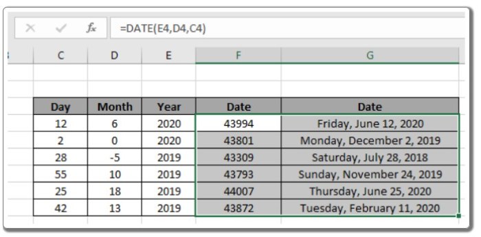

As you can see from the snapshot, the DATE function takes the day, month, and year values as input and returns the complete date value. Negative or zero values as arguments will shift the date accordingly.

The DATE function in Excel is often used in combination with other logical functions to calculate date values. For example, you can extract the month, day, and year from a date to perform further calculations, as shown in the example below to get the next anniversary date.

Use the formula: =DATE(YEAR(D5) + 1, MONTH(D5), DAY(D5))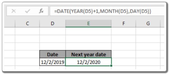

Here, the DAY function extracts the day, the MONTH function extracts the month, and the YEAR function extracts the year value from the date. These values are then used as arguments in the DATE function to return the required date value.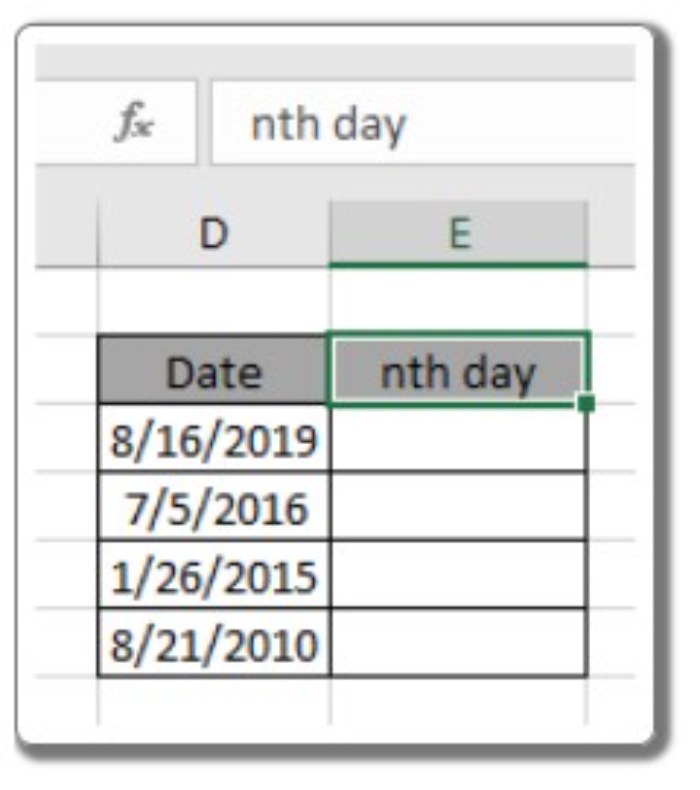

You can also use the DATE function to find the nth day of the year from a given date. Here’s how you can do it: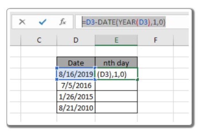

Use the formula: =D3 – DATE(YEAR(D3), 1, 0)

Explanation: The YEAR function returns the year value of the given date. The DATE function takes the year value as an argument and returns the last date of the previous year. The subtraction operator calculates the difference between the two dates and returns the elapsed date.

You can use the above formulas to calculate the number of days between dates in Excel.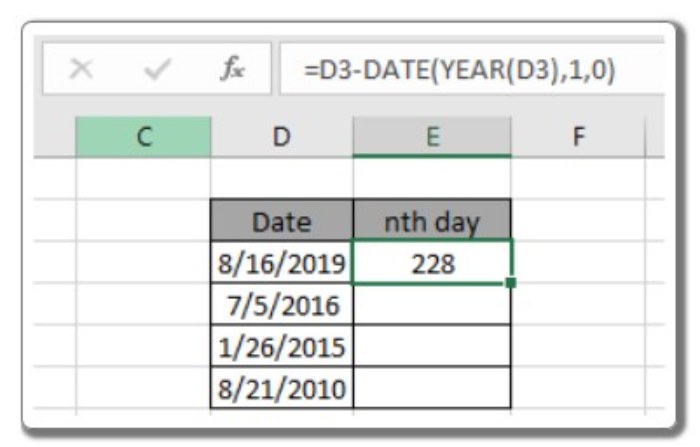

As you can see, the formula works fine and returns 228 as the result. Now you can drag the formula down to apply it to the remaining dates in the dataset.

Here are the days from the year calculated using the formula.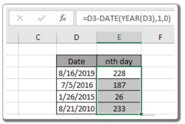

We can achieve the same result using an alternative approach. By subtracting the given date value from the first date of the same year and adding 1, we can calculate the elapsed days. The generic formula is as follows: = date – DATE(YEAR(date), 1, 1) + 1

Both formulas yield the same result, so you can choose whichever one you prefer. However, it’s important to note that you should not directly input the date argument into the formula. Excel formulas may not always understand the date value and could return an error. Instead, provide the date argument using the DATE function or by referencing a cell.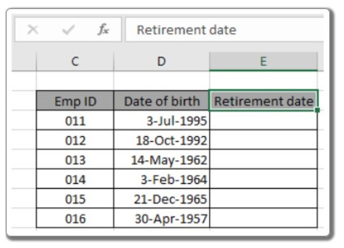

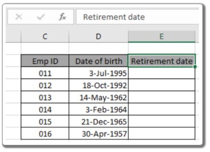
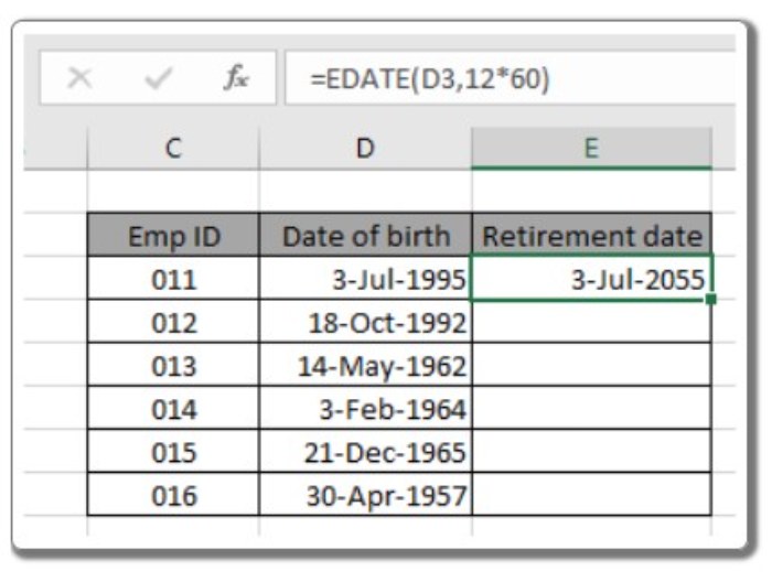
Now let’s consider an example using the EDATE function. Suppose we have a list of birth dates with corresponding employee IDs. Our goal is to determine the retirement date based on the given birth dates.

To calculate the retirement date, use the formula in cell E3: =EDATE(B3, 12*60)

How to use the DATE function in Excel

In this formula, the date value is referenced from cell B3. Press Enter to obtain the retirement date.

How to use the DATE function in Excel

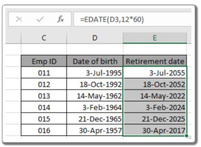
As you can see, the retirement date for employee ID 011 is July 3rd, 2055. To apply the formula to other cells, you can use the drag-down option or the shortcut key Ctrl + D, as shown below.

How to use the DATE function in Excel

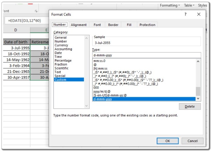
By utilizing the Excel EDATE function, we have successfully obtained the retirement dates for all employees. However, please note that the returned date values might not be in the desired format. To format the cells accordingly, you can use the format cell option or Ctrl + 1, as demonstrated in the snapshot below.

How to use the DATE function in Excel

Here are some additional notes to consider:

• The formulas only work with numeric values.
• The arguments provided to the function must be numeric; otherwise, the function will return a #NAME? error.
• Not providing any arguments to the function will result in a #NUM! error.
• If no year argument is specified, the year value defaults to 1900.
• The MONTH and DAY arguments can be zero or negative. For example, using 1 as the day argument will return the first day of the month, while a 0 input will return the last date of the previous month.