Tips for mastering how to calculate square roots in Excel

What is the method for inputting square roots in Excel? How do you calculate square roots in Excel? These are basic questions that many people have been searching for recently. In this article, Buffcom.net will give you tips for mastering how to calculate square roots in Excel.
For arithmetic operations such as addition, subtraction, multiplication, and division in Excel functions, we mostly know how to use and perform them. However, for operations involving exponents and calculating square roots in Excel, they are less commonly used. So, in Excel functions, how do we calculate square roots, cube roots, and write exponents? Let’s find out with Buffcom.net in this article.
I. Instructions for calculating square roots in Excel with the SQRT function
1: How to write exponents in Excel

How to calculate the square root in Excel
In mathematics, exponents are usually written in the form:
In cell A1, we see the digit 2 written smaller and above and to the right of the letter A.
In cell A2, we see the digit 2 written horizontally and separated from the letter A by the exponent symbol ^ (press shift + 6).
In both ways of writing, we understand that it is A raised to the power of 2. However, in Excel functions, the way of writing in cell B1 is used to calculate and produce the result. The way of writing in cell A1 is just for presentation purposes in text format.
For example:
In cell A3, when we enter the number 42 as TEXT (with a single quotation mark (‘) before the number 4), we can then select the Format Cells option, format the number 2 as Superscript.
In cell A4, we will write =4^2 to get the result of 16.
So, the method for writing exponents in Excel is A raised to the power of n = A^n.
2: How to write square root in Excel
Unlike exponentials, square roots can be written in Excel using the following formula: square root in Excel of A = A^(1/2)
For example:
Square root in Excel of 16 is 16^(1/2) = 4
Thus, the general formula is:
nth root of A = A^(1/n)
Cube root of A = A^(1/3)
Fifth root of A = A^(1/5)
3: SQRT function in Excel
In addition to the above formula, Excel also has a specific function called SQRT to calculate square roots. The syntax is:
SQRT(number) is the function to calculate the square root of a number in Excel. Note that this function only works for square roots and cannot be used for other types of roots.
II. How to calculate square root in Excel using operators

How to calculate square root in Excel using a formula
When doing manual calculations, square roots are written using the symbol (√). Although this symbol cannot be entered in traditional Excel, there is a way to find square roots in Excel without using any functions. For this, use the caret (^) symbol, which is located above the number 6 on most keyboards.
In Excel, the caret (^) symbol is used as an exponent operator. For example, to square the number 5, you would enter = 5 ^ 2 in a cell, which is equivalent to 5 squared.
To find the square root in Excel, use the caret operator with (1/2) or 0.5 as the exponent:
Number ^ (1/2) or Number ^ 0.5
For example, to find the square root in Excel of 25, you would enter = 25^(1/2) or = 25^0.5 in a cell.
To find the square root of a number in cell A2, you would enter: = A2^(1/2) or = A2^0.5
The SQRT function in Excel and the exponent formula provide the same result:
This square root formula in Excel can be used as part of larger formulas. For example, the following IF statement requires Excel to calculate the square root under certain conditions. It returns the square root if cell A2 contains a number, but returns a blank string (empty cell) if A2 is a text value or blank.
=IF(ISNUMBER(A2), A2^(1/2), “”) can be translated to “If A2 is a number, return the square root of A2, otherwise return an empty string.”
The reason why the exponent of 1/2 is equivalent to the square root is because the square root of a number is the same as raising that number to the power of 1/2.
To start, let’s call the square root function in Excel as what it is: a number that, when multiplied by itself, equals the original number. For example, the square root of 25 in Excel is 5 because 5 x 5 = 25.
Multiplying 25 to the power of 1/2 by itself also gives 25: 25 ½ x 25 ½ = 25 (½ + ½) = 25 (1) = 25.
In other words: √25 x √25 = 25 and 25 ½ x 25 ½ = 25.
Therefore, 25 ½ is equivalent to √25.
III. Square Root with the POWER Function
1: How to Calculate Any Root

quare root in Excel using Power function
The exponent formula above is not limited to finding only the square root in Excel. Similarly, it can be used to find any nth root by simply inputting the desired root value in the denominator of a fraction after the caret symbol:
Number ^ (1/n)
Where the number is the value you want to take the root of and n is the root’s power.
2: Using the POWER Function
The POWER function is just another way to perform the same calculation, i.e., raising a number to the power of 1/2.
The formula for the POWER function in Excel is written as:
POWER(number, power)
As you can easily guess, to get the square root, you need to provide 1/2 as the power argument. For example:
=POWER(A2, 1/2)
As shown in the image below, all three formulas for the square root in Excel produce the same result. Which one to use is a matter of personal preference.
IV. Components of Microsoft Excel Formulas
1: Operators in Excel Spreadsheets
To tell Microsoft Excel software what type of task you want to perform in a formula, use special symbols called operators. There are four types of operators in Excel:
Arithmetic – to perform basic arithmetic operations.
Comparison (logical) – used to compare values.
Concatenation – used to combine text values into a single string.
Reference – used to create cell ranges and separate arguments in Excel functions.
2: Using Arithmetic Operators in Excel Formulas

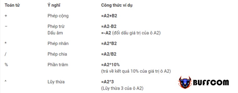
Using square root operators in Excel
These operators are used to perform basic arithmetic operations such as addition, subtraction, multiplication, and division.
3: Comparison Operators in Excel Formulas
In Microsoft Excel formulas, comparison, or logical, operators are used to compare two values. The result of a comparison is always a logic value of TRUE or FALSE. The following logical operators are available in Excel:

Square root operators in Excel
For example, the formula = A1 = B1 will return TRUE if cells A1 and B1 have the same value (number, text, or date), and FALSE if they do not.
4: Concatenation Operator
The operator used to concatenate text in Excel is the ampersand symbol (&). You can use it to combine two or more text strings into a single string.
For example, if you have a country code in column A and a phone number in column B, you can use the following formulas to get the phone number combined with the country code:
= A1 & “” & B1
In the formulas above, we add a space in between to make the numbers more readable:
The same result can be achieved using the CONCATENATE function.
5: Reference Operators in Excel Formulas and Functions
To provide data ranges to MS Excel formulas and for separate arguments in Excel functions, the following operators are used.
Colon (:) – this is a range operator that allows you to create a reference to multiple cells between two cells you specify.
For example, the range A1:A100 includes 100 cells from A1 to A100. To find the average of these 100 cells, use the following formula: = AVERAGE (A1:A100)
You can also refer to entire columns (A:A) or entire rows (1:1). For example, the following formula can find the sum of all numbers in column A: = SUM (A:A).
Comma (,) – is used to separate arguments in Excel spreadsheet formulas. For example, the formula =IF(A1>0, “good”, “bad”) reads as follows: if A1 is greater than zero, return “good”, otherwise “bad”.
Note: The comma is a default separator in North America and some other countries. In European countries, the comma is reserved as a decimal symbol, and the separator marks are typically replaced with semicolons (;). In this case, if you need to separate the arguments with semicolons, for example: =IF(A1>0; “good”; “bad”).
Therefore, if you are trying to create a formula in your spreadsheet, but Excel does not accept it and gives an “invalid formula” error, go to Regional Settings (Control Panel> Region and Language> Additional Settings) and check which separator is set as the decimal symbol there. That may be the separator you need to use to distinguish the arguments in your Excel formula.
Whitespace – it is an operator for intersection that allows you to retrieve the values at the intersection of two specified references. For example, if you have a list of items in column A and some related data in other columns, you can get the values at the intersection of a column and row by using the formula like this: =B3:D3 C2:C4.
V, Tips and Shortcuts to Save Time for Excel Formulas

Tips on quadratic formula in Excel
Excel formulas are a powerful and versatile tool that can solve many tasks in your spreadsheets. Of course, learning the different aspects of Excel functions and formulas can take a lot of time. So you may feel like you don’t have enough time to learn everything. Well, one good way to find more time is to save time.
To switch between absolute, relative, and mixed references in the same formula, use the F4 key.
To review all the formulas on the worksheets, click the Show Formulas button on the Formulas tab > Formulas Auditing group, or press Ctrl + ~.
To edit a formula, press F2, or double-click a cell, or click on the formula bar.
To debug a formula error in Excel, select a portion of the formula and press F9. This allows you to see the actual values behind the cell references.
To copy a formula to almost all cells in the same column, enter the formula in the first cell, select that cell and drag the small square at the bottom right corner until it becomes a black cross (called the Fill handle). Double-click on that cross and you get the formula copied throughout the column.
To convert formulas to values, select all the cells with the formulas you want to convert, press Ctrl + C to copy them, then press Shift + F10, then press V, and then press Enter. Shift + F10 + V is the shortcut for Excel’s special Paste Values. If you are not sure you will remember this shortcut, just press the usual shortcut to paste, Ctrl + V, click the small arrow to the right of the Paste button to open the drop-down list and select Paste Values.
To use Excel effectively in your work, you need to not only master the functions but also be good at using Excel tools. Advanced functions like SUMIFS, COUNTIFS, SUMPRODUCT, INDEX + MATCH will help you apply well to your work. These tools often use Data validation, Conditional formatting, Pivot table…
In conclusion, Buffcom.net has provided you with skills and Excel tips and tricks in general, and quadratic functions in Excel in particular. With the above suggestions, we hope that you can easily apply them in your life and work. Buffcom.net wishes you success.


