• Microsoft Office
  • Microsoft Windows
  • Other Software
  • Anti Virus
  • Blog
    • Word
    • Excel
    • Powerpoint
    • Software tricks/tips
  • POLICIES
    • PAYMENT GUIDE
    • SHIPPING POLICY
    • REFUND POLICY
    • TERMS & CONDITIONS
    • Contact Us

No products in the cart.

  • Microsoft Office
  • Microsoft Windows
  • Other Software
  • Anti Virus
  • Blog
    • Word
    • Excel
    • Powerpoint
    • Software tricks/tips
  • POLICIES
    • PAYMENT GUIDE
    • SHIPPING POLICY
    • REFUND POLICY
    • TERMS & CONDITIONS
    • Contact Us

No products in the cart.

  • Microsoft Office
  • Microsoft Windows
  • Other Software
  • Anti Virus
  • Blog
    • Word
    • Excel
    • Powerpoint
    • Software tricks/tips
  • POLICIES
    • PAYMENT GUIDE
    • SHIPPING POLICY
    • REFUND POLICY
    • TERMS & CONDITIONS
    • Contact Us

No products in the cart.

  • Microsoft Office
  • Microsoft Windows
  • Other Software
  • Anti Virus
  • Blog
    • Word
    • Excel
    • Powerpoint
    • Software tricks/tips
  • POLICIES
    • PAYMENT GUIDE
    • SHIPPING POLICY
    • REFUND POLICY
    • TERMS & CONDITIONS
    • Contact Us
Excel

Detailed instructions for drawing a pie chart in Excel

0 Comments

Detailed instructions for drawing a pie chart in Excel: A pie chart is a visual display that allows you to see the relationship of each part to the whole data (usually as a percentage). Especially if you use Excel to track, edit, and share data, drawing a pie chart will be very reasonable. This article will guide you on how to draw a pie chart in Excel.

1. Prepare the data

Unlike other types of charts, a pie chart in Excel requires the data to be arranged in a column or row. Therefore, each chart represents only one type of data. You can add category names to the column or row, and it should be the first column or row in the selection range. Category names will appear in the chart legend or chart title.
Note:

  • There is only one data series, if there are more than 1 series that you still want to draw in pie chart form, you can choose the Doughnut chart.
  • No value in the data carries a negative value.
  • No value in the data has a value of zero (or empty), if so, that value will not be displayed in the pie chart.
  • No more than 7 data components, because too many parts will make your chart difficult to understand.
Detailed instructions for drawing a pie chart in Excel

Detailed instructions for drawing a pie chart in Excel

2. Draw a pie chart using Smart tag

To create a chart using Smart tag, you just need to highlight the entire data table. At this point, the Smart tag icon will appear in the lower right corner of the data table. Click here and select the Charts => Pie option.

Detailed instructions for drawing a pie chart in Excel

Detailed instructions for drawing a pie chart in Excel

Just like that, you have basically drawn a pie chart representing the data in the table.

Detailed instructions for drawing a pie chart in Excel

Detailed instructions for drawing a pie chart in Excel

3. Create a regular pie chart

Detailed instructions for drawing a pie chart in Excel

Detailed instructions for drawing a pie chart in Excel

You highlight the entire data table, then select the Insert tab on the toolbar. Next, click on the Insert Pie chart icon in the Charts section. The scroll bar appears, then you select the chart template you want to create.

That’s it, the pie chart representing the data in the table has been successfully created.

Detailed instructions for drawing a pie chart in Excel

Detailed instructions for drawing a pie chart in Excel

4. Customize the pie chart.

After you have finished drawing the pie chart. You need to perform some customization to make your chart more scientific and impressive.
a. Edit the title of the pie chart.
Double-click the title and edit the appropriate title for the pie chart.

Detailed instructions for drawing a pie chart in Excel

Detailed instructions for drawing a pie chart in Excel

b. Move and resize the pie chart.
Press and hold the left mouse button on the pie chart and drag it to where you want to move the chart.

To resize the chart, you can click and drag one of the handles on the chart’s edge. You can also right-click on the chart and select the Format Chart Area option to adjust the size and position of the chart.

Detailed instructions for drawing a pie chart in Excel

Detailed instructions for drawing a pie chart in Excel

c. Add data labels to a pie chart.
Click on the “+” icon next to the pie chart. Then tick the box next to “Data Labels”, and the data labels will appear.

Detailed instructions for drawing a pie chart in Excel

Detailed instructions for drawing a pie chart in Excel

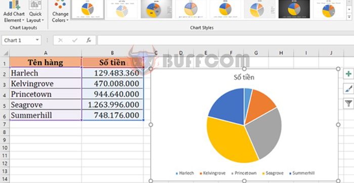
d. Change the chart type.
You can change the style and color of your chart with many options. To access each of the following items, click on the chart, select “Chart Styles”, and then make your selection.

Detailed instructions for drawing a pie chart in Excel

Detailed instructions for drawing a pie chart in Excel

Thus, the above article has guided you on how to create a pie chart in Excel. We hope this article will be useful to you in your work. Wish you success!

9
61 Views
8 Default Word Settings to Configure Before ComposingPrev8 Default Word Settings to Configure Before ComposingMarch 22, 2023
How to create Up/Down button for Excel spreadsheetMarch 22, 2023How to create Up/Down button for Excel spreadsheetNext

Leave a Reply Cancel reply

Your email address will not be published. Required fields are marked *

Recent Posts
  • Retrieve Data Based on Data Validation
    September 7, 2023
    Excel
  • How to Convert Multiple Rows to Columns and Rows in Excel?
    September 6, 2023
    Excel
  • VLOOKUP for Automatic Discount in Data Validation
    September 6, 2023
    Excel
  • How to Convert Text Dates to Dates in Excel?
    September 5, 2023
    Excel
Categories
  • Blog 80
  • Excel 754
  • Powerpoint 36
  • Software tricks/tips 128
  • Uncategorized 8
  • Word 109
Tags
the ISERROR
Top rated products
  • Trend Micro Internet Security 3 Devices 1 Year Key GLOBAL Trend Micro Internet Security 3 Devices 1 Year Key GLOBAL
    Rated 5.00 out of 5
    $17.00
  • Windows 11 Pro Key Global
    Rated 5.00 out of 5
    $11.00
  • AVG Internet Security 2021 10 Devices 2 Years Global AVG Internet Security 2021 10 Devices 2 Years Global
    Rated 5.00 out of 5
    $42.20
  • Trend Micro Maximum Security 3 Devices 1 Year key Global Trend Micro Maximum Security 3 Devices 1 Year key Global
    Rated 5.00 out of 5
    $15.00
  • Windows 11 Home Key Global 2021
    Rated 5.00 out of 5
    $15.00
Products
  • Buy Office 2021 Professional Plus Key Global For 5 PC
    Rated 5.00 out of 5
    $45.00
  • Buy Office 2021 Professional Plus Key Global Bind To Your Microsoft Account
    Rated 4.83 out of 5
    $49.00
  • Windows Server 2022 Datacenter Key Global
    Rated 5.00 out of 5
    $15.00
  • Windows Server 2022 Standard Key Global
    Rated 4.47 out of 5
    $15.00
  • Windows Server 2022 Remote Desktop Services Device Connections (50) Cal Key Global
    Rated 5.00 out of 5
    $45.00

Buffcom.net always brings the best digital products and services to you. Specializing in Office Software and online marketing services

BIG SALE 50% IN MAY

Microsoft Office
Microsoft Windows
Anti-Virus
Contact Us

Visit Us:

125 Division St, New York, NY 10002, USA

Mail Us:

buffcom.net@gmail.com

TERMS & CONDITIONS | PAYMENT GUIDE  | SHIPPING POLICY  | REFUND POLICY

Copyright © 2019 buffcom.net  All Rights Reserved.