Effective use of the IFERROR function in Excel

Effective use of the IFERROR function in Excel In Excel, you have the ability to catch errors by utilizing the iferror function. With the use of parameters, you can customize what value is returned when specific errors occur.
This article will teach you how to effectively handle and evaluate errors in Excel with the iferror function. Among the types of errors that can be handled include #n/a, #value!, #ref!, #div/0!, #num!, #name?, or #null! errors.

Mastering the Syntax of IFERROR Function in Excel

Let me show you the syntax of the iferror function:

IFERROR(value, value_if_error)

As mentioned earlier, the iferror function requires two inputs: the value and the value_if_error. The value parameter represents the input that needs to be examined for an error, while the value_if_error parameter determines what will be returned if an error occurs. The following examples will clarify the function of these parameters.

Mastering the IFERROR Function in Excel

In this section, we will demonstrate a practical use case for the IFERROR function.

The table below will be the basis for our illustration.

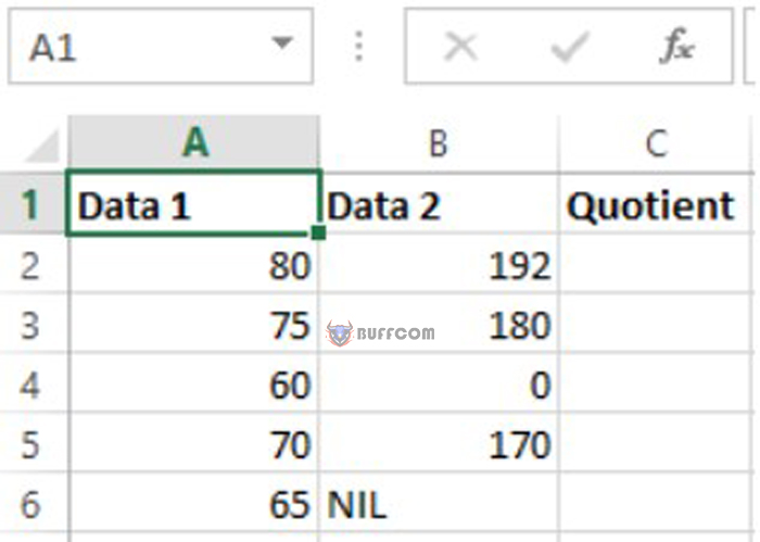The table displayed contains three columns: Data 1, Data 2, and Quotient.

The objective is to compute the values of the Quotient column by dividing Data 1 by Data 2.

For instance, in row one, we divide 80 by 192, and in row two, we divide 75 by 180, and so forth. However, upon close inspection, certain rows have values that will produce errors in mathematical calculations – rows 4 and 6. In row 4, we cannot divide 60 by zero, and in row 6, we cannot divide 65 by nothing.

The resulting table after performing the divisions will appear as follows:

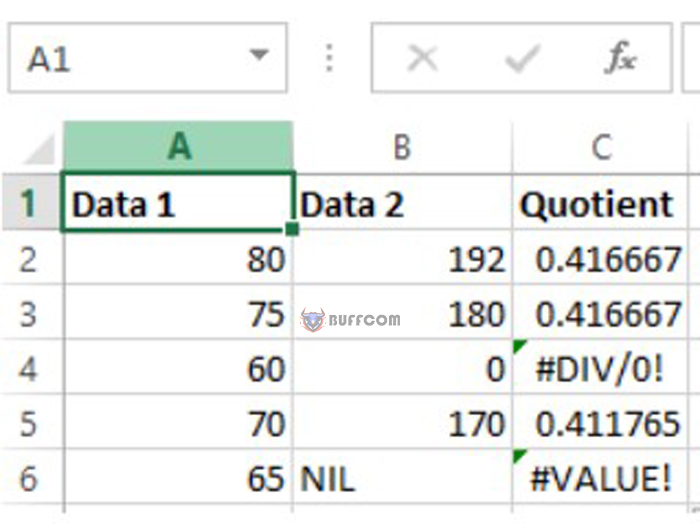Column 4 and 6 produce errors while performing mathematical operations and display #div/0! and #value!, respectively. Although we cannot resolve these math errors, we can intercept them to display a custom value. To do this, we can use the iferror function.

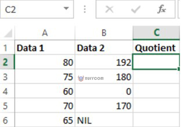After deleting all values in the quotient column, the subsequent step is to apply the iferror function which goes as follows:

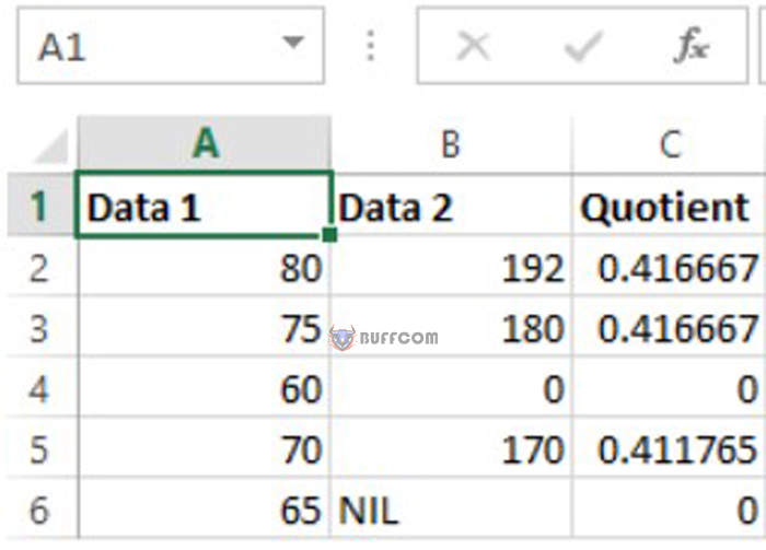
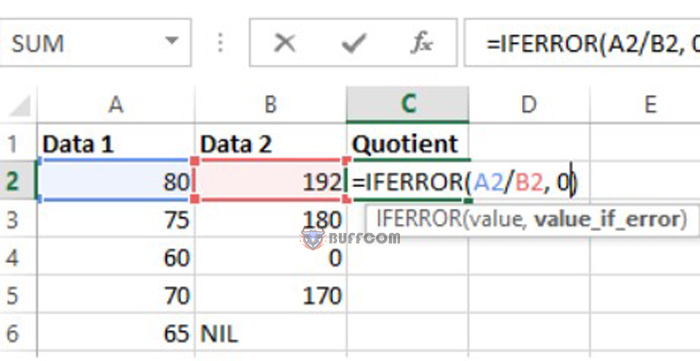We added an “iferror” function in the first row of the table. The function is “=iferror(a2/b2, 0)” and has two parameters.

The quotient for row 4 and 6 has been updated to 0, replacing the previous values of #div/0! and #value!, respectively.

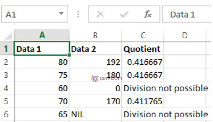
It’s worth mentioning that you can also utilize a customized message instead of 0, such as =iferror(a2/b2, “division not possible”). Just make sure to enclose the text in quotation marks. As a result, our table will now look like this:

You have the flexibility to personalize what will be displayed in case of an error.

In this article, we discussed the iferror function in Excel, which effectively manages various errors such as #n/a, #value!, #ref!, #div/0!, #num!, #name?, and #null!. We examined the proper syntax and the significance of its parameters, as well as providing examples of how to utilize the iferror function in an Excel table. Thank you for taking the time to read!