Excel Conditional Formatting Based on Another Column

Excel Conditional Formatting Based on Another Column. Sometimes, you may need to format cells or columns in Excel based on the values in another column. If you’re in such a situation, this guide will show you how to format cells based on another column’s values using an example.

Example: Highlighting months with sales higher than the average

Let’s say we have data on sales made by different dealerships in different months and years. We want to highlight sales in 2019 that are greater than sales in 2018.

To achieve this, follow these steps:

1. Select the range D2:D12 (sales of 2019).
2. Go to the Home tab, click on Conditional Formatting, and select New Rule.
3. In the New Formatting Rule dialog box, choose “Use a formula to determine which cells to format.”
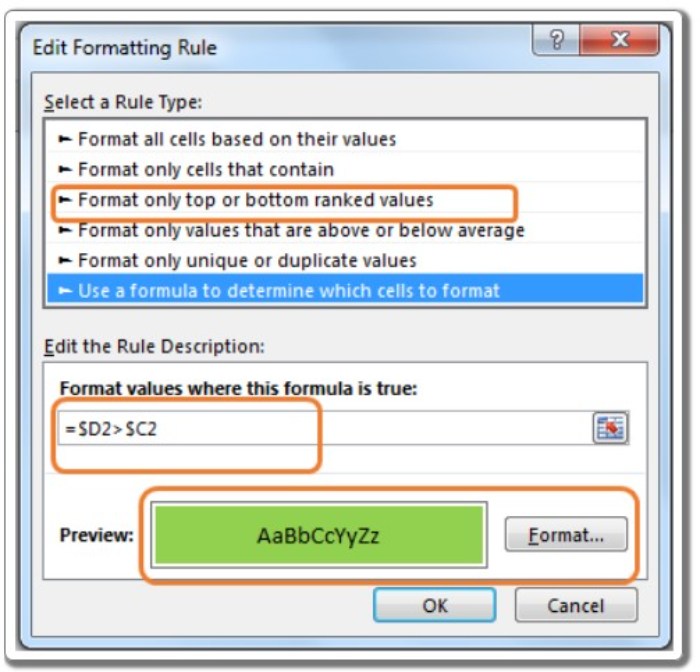
4. In the formula box, enter the following formula for Excel formatting: =$D2>$C2
5. Select the formatting you want for cells that meet the condition. In this example, we will choose a green fill.
6. Click the OK button.

That’s it! All the values in the 2019 sales column that are greater than the corresponding values in the 2018 sales column will be highlighted with a green fill.

How does it work?

It’s simple. First, you select the range where you want the formula to apply. Then, you use a formula to determine which cells within that range should be formatted. In this case, the formula is $D2>$C2. The dollar sign ($) locks the column reference (D) while allowing the row reference (2) to change as the formatting is applied to other cells. The formula compares each cell in the range (D2:D12) with the corresponding cell in the previous year’s sales column (C2:C12). If a cell in 2019 sales is greater than the corresponding cell in 2018 sales, it will be formatted with the chosen style (green fill).

If you want to highlight the months instead of the 2019 sales, you can directly change the “applies to” range to A2:A12.

1. Select any cell in the range D2:D12.
2. Go to Conditional Formatting and click on “Manage Rules.”
3. Change the range in the “Applies to” box to A2:A12.
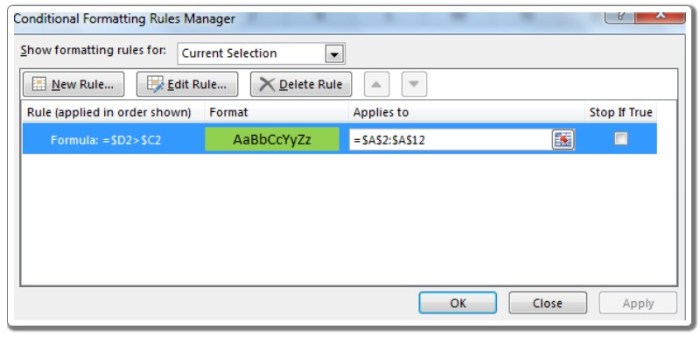
4. Click the OK button.

You will see that the formatting is now applied to the specified range. Similarly, you can format any range based on the values in any column in Excel. The column can even be on a different sheet; you just need to mention the range. You can also specify non-contiguous ranges by using commas between the ranges in the “applies to” section.

So, this is how you can apply conditional formatting in Excel based on another column. It might seem a bit tricky, but in practice, it’s quite straightforward. You just need to make a few adjustments. I hope this article has provided enough explanation to help you with conditional formatting in Excel. If you have any doubts, feel free to mention them in the comments section below.