How to Convert Columns to Rows (and Vice Versa) in Excel

If you want to convert columns to rows or vice versa in Excel, you can use the TRANSPOSE function. This function allows you to easily change the orientation of your data. Follow these steps to convert columns to rows:

How to Convert Columns to Rows (and Vice Versa) in Excel

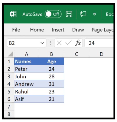
1. Select a range of cells where you want to place the transposed data. For example, let’s say you have a list of names in column A and corresponding ages in column B, and you want to convert this into rows.
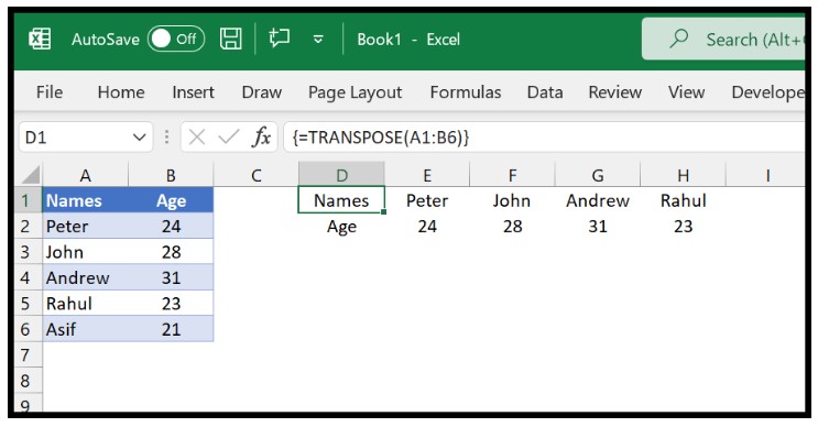
2. In the selected range, enter the TRANSPOSE function. For example, if you want to transpose the data from columns A and B, enter “=TRANSPOSE(A1:B6)” in the range.
3. After entering the TRANSPOSE function, close the parentheses and press and hold the CTRL + SHIFT keys.
4. Finally, press the ENTER key while still holding the CTRL + SHIFT keys. This combination of keys is important to activate the array formula.

The TRANSPOSE function will convert the vertical cells into horizontal cells, effectively changing columns to rows.

It’s worth noting that the TRANSPOSE function requires you to select the same number of cells in the opposite orientation. Also, remember to use CTRL + SHIFT + ENTER to apply the function correctly.

Once the transposed data is created, it will be linked to the original data. So if you change a value in any of the cells from the original range, the corresponding value in the transposed range will also be updated.

If you want to convert the transposed range into values and disconnect it from the original data, you can use the “Paste Special” function or use the keyboard shortcuts Ctrl + C to copy the range and then Alt + V, followed by V to paste values only.

By following these steps, you can easily convert columns to rows or vice versa in Excel using the TRANSPOSE function.