How to Display Negative Values in Parentheses in Excel

To make negative numbers look neater and more visually appealing during data processing, this article will guide you on how to display negative values in parentheses in Excel. Let’s take a look together!

Example of displaying negative values in parentheses:

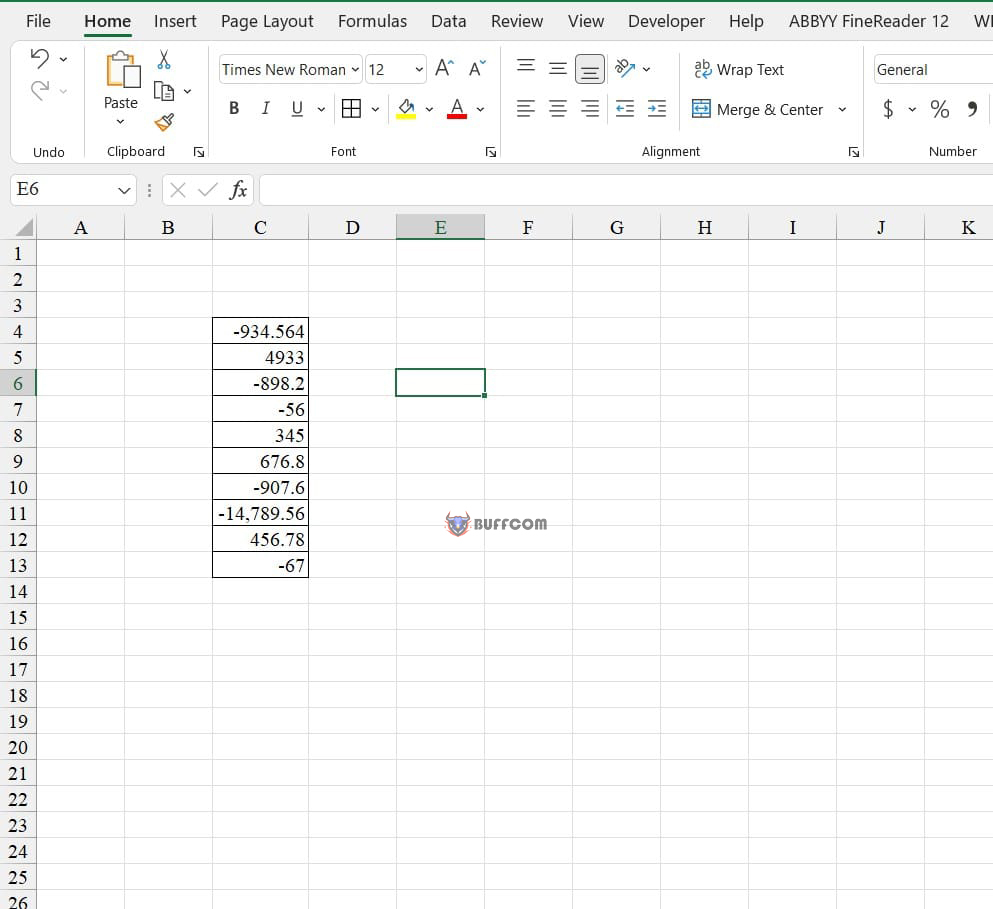
Assuming we have the following data:

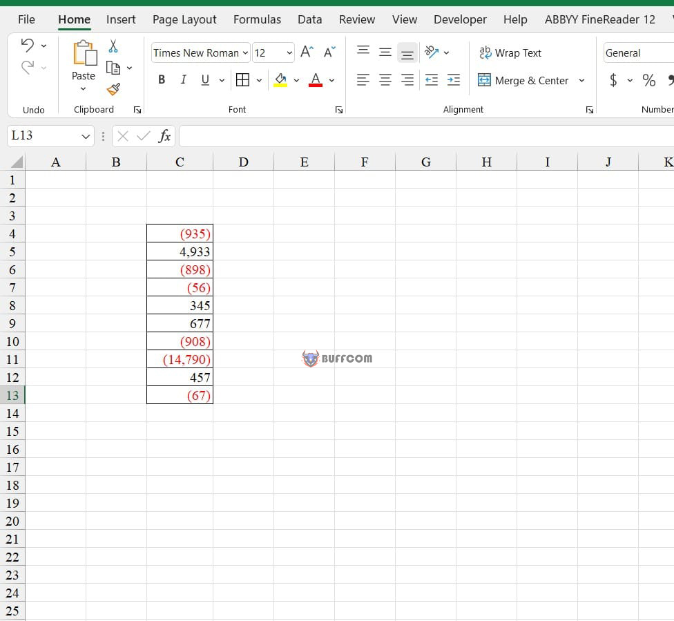
The requirement is to display negative numbers in parentheses, with the negative value in red font.

To do this, follow these steps:

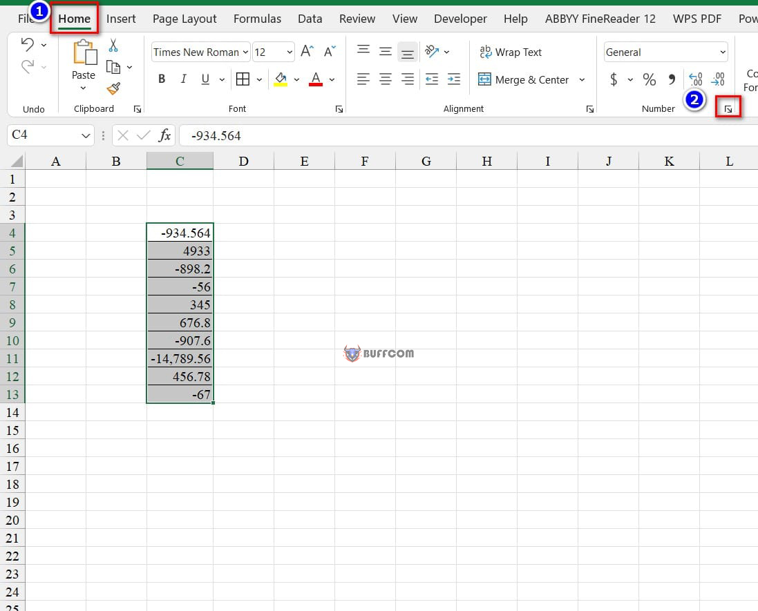
Step 1: Select the data range.

Step 2: On the Home tab, click on the arrow on the right side of the Number group.

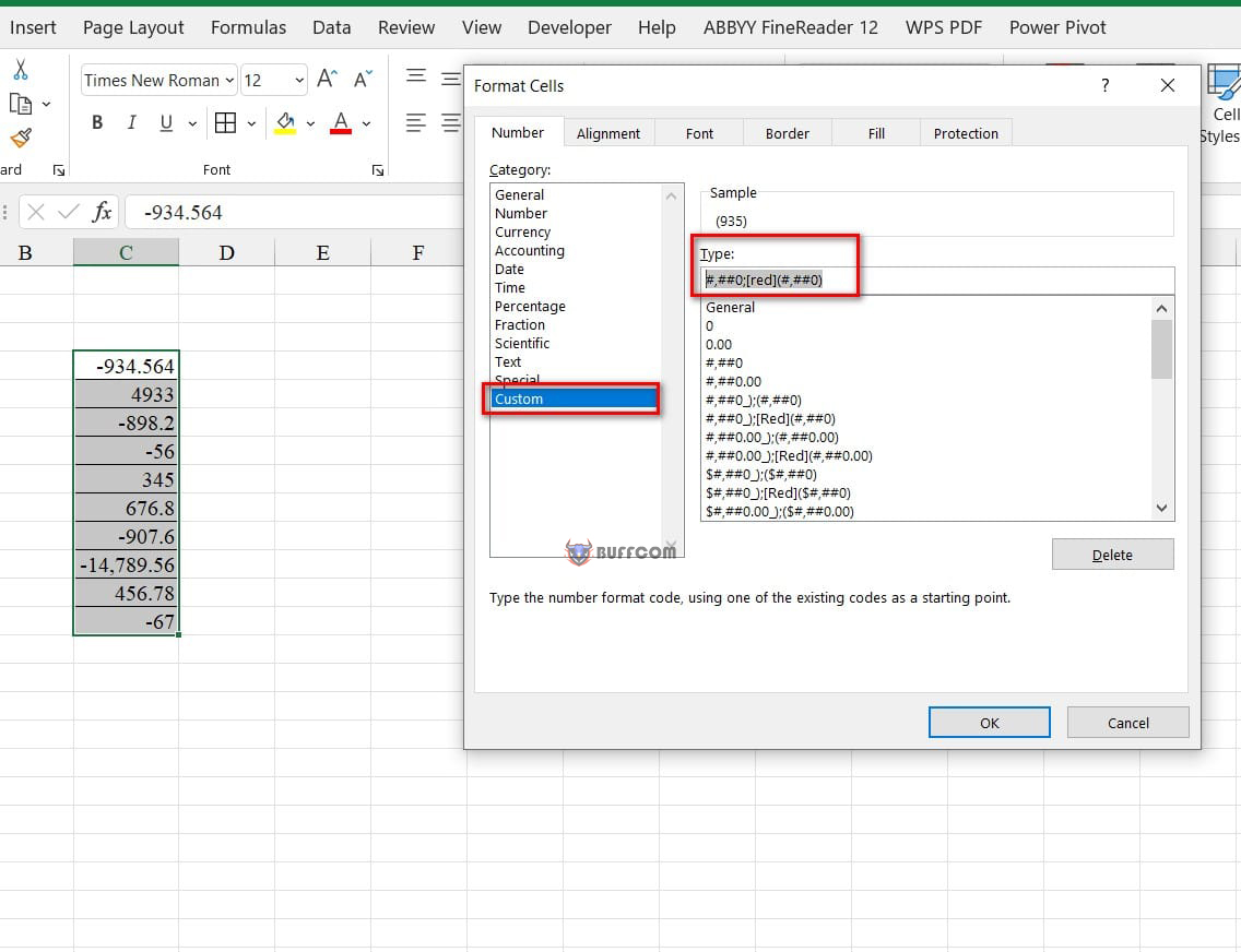
Step 3: In the Format Cells dialog box, select the Custom category, and then in the Type field, enter “#,##0;red”.

Step 4: Click OK to complete.

To modify the display format: Select the data range, click on the arrow on the right side of the Number group again. In the Format Cells dialog box, modify the requirements in the Type field.

That’s it! We have just guided you on how to display negative values in parentheses in Excel. We hope this article will be helpful to you, and if you find it useful, please don’t forget to rate the article below!