How to Use Conditional Formatting to Improve Readability of Larger Values in Excel

How to Use Conditional Formatting to Improve Readability of Larger Values in Excel. In order to enhance the readability of large values in Excel, you can utilize conditional formatting. This article demonstrates how to apply a custom format that makes larger values easier to read. For instance, instead of displaying 1,200,000 as is, it can be formatted as 1.2 M, which not only rounds the value but also uses a more readable format. However, when dealing with values less than a million, the custom format still includes the “M” for million but drops the decimal point. For example, 669,227 is displayed as .67 M. Realistically, this format isn’t significantly more readable than the original value and could be easily misinterpreted. Therefore, this article presents two conditional formatting rules in Excel that abbreviate large values, one for millions and another for thousands.

How to Use Conditional Formatting to Improve Readability of Larger Values in Excel

Excel’s Custom Millions Format:

Let’s examine the custom format used in the aforementioned article:

$#.##,,” M”;

The format consists of four sections separated by semi-colons (;). However, we will only focus on the first section, which applies to positive values. Nonetheless, let’s provide an explanation of all four sections:

1. First section: Applies to positive values.
2. Second section: Applies to negative values.
3. Third section: Applies to zero.
4. Fourth section: Applies to text.

Now, let’s break down the custom format we’ll use for values equal to or larger than one million. This format includes the dollar symbol, “$,” on the left side. Next, “#.##,,” handles the actual digits. The two commas represent the thousands separator, and “,,” omits values in the thousands and hundreds places. For instance, 1,780,379 is displayed as $1.78 M. The decimal point is necessary for proper conversion, as 1.78 M is not the same as 178 M.

To add this custom format to your Excel workbook, follow these steps:

1. On the Home tab, click on the dialog launcher for the Value group.
2. If necessary, click on the Value tab.
3. In the Category list, select Custom.
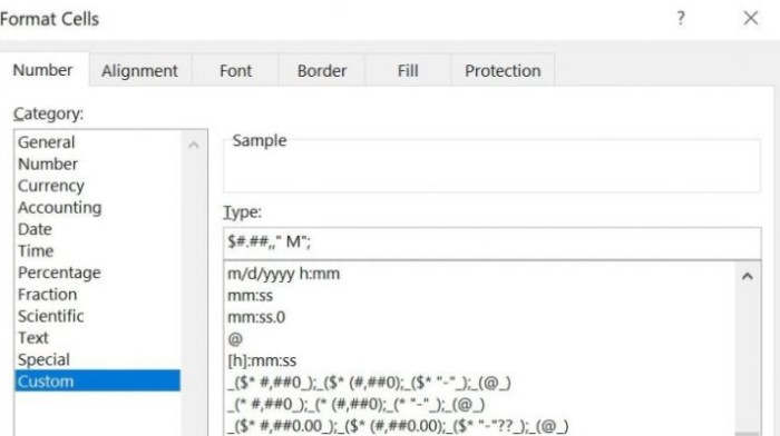
4. In the Type control on the right, enter the custom format “$#.##,,” M” (as shown in Figure A).
5. Click OK.

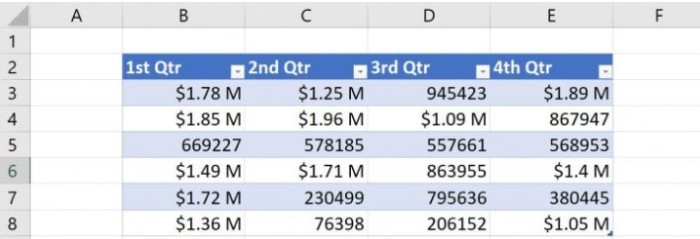
The resulting custom format will be applied, as displayed in Figure B. Notice that this format only affects the visual representation of the value, not the underlying data. However, you may find that values less than one million are not as readable as desired and may even be misread. Therefore, a custom thousands format is necessary.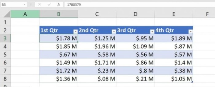

Excel’s Custom Thousands Format:

At this point, you can attempt to create the custom thousands format yourself. If you came up with “$###, K”, you are correct! The important component to notice is “###,” which represents the three possible digits in the thousands position and omits the digits in the hundreds position. Additionally, “K” is commonly used to denote thousands, making it a suitable choice. Follow the instructions above to add this custom format. Once both custom formats are added, it’s time to create the conditional formatting rules to apply them.

Creating Conditional Formatting Rules in Excel:

After creating the custom value formats, you can apply them using conditional formatting rules. Currently, the format is set to General. Begin by selecting the data set shown in Figure C.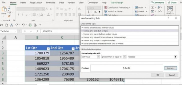

To create an Excel conditional format rule that handles values greater than or equal to one million, follow these steps:

1. Select the data set (B3:E8).
2. On the Home tab, click on Conditional Formatting in the Styles group.
3. Choose New Rule from the dropdown list.
4. In the resulting dialog, select

Format Only Cells That Contain in the top pane.

5. In the lower pane, choose “Greater Than or Equal to” from the second dropdown (the first dropdown should be set to “Cells”).

1. In the third control, enter “1000000”.
2. Click Format.
3. Go to the Number tab.
4. From the Category list, select Custom.
5. On the right side, choose the custom format “$#.##,,” M” (refer to Figure D).
6. Click OK.

Figure D demonstrates the selection of the custom millions format. Click OK to apply the rule. As shown in Figure E, only values greater than or equal to one million will be formatted accordingly.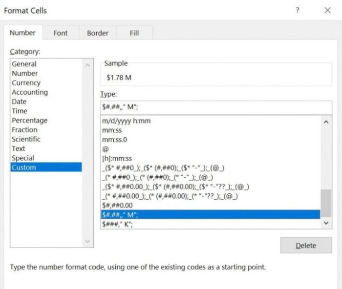

Now, repeat the instructions to add a rule for the custom format “$###, K” (refer to Figure F for steps 6 and 10).

Figure F represents the addition of the second conditional formatting rule.

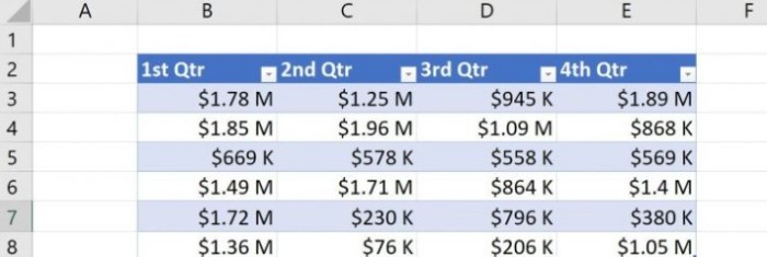
Figure G displays the results, with both custom formats applied to all the values. If your dataset contains values in the trillions or below a thousand, you can create new custom formats for those positions and apply them using conditional formatting. Excel can handle various formats for improved readability.

Figure G