How To Use Slicer In Excel – A Data Filtering Tool

Slicer in Excel is an extremely powerful data analysis tool used to filter data based on specific criteria. This feature is commonly used with traditional spreadsheets or Pivot Tables. In this article, Buffcom.net will share how to use this useful Slicer feature.

Introduction to Slicer Feature in Excel

The Slicer feature is integrated into the Pivot Table tool. It is used to filter data based on a specific field in the table and then create a report based on the filtered data.

You can understand it better through the following example:
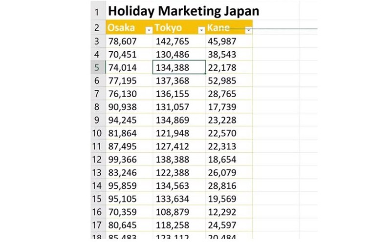
This is a data table with three fields: Osaka, Tokyo, and Kane.

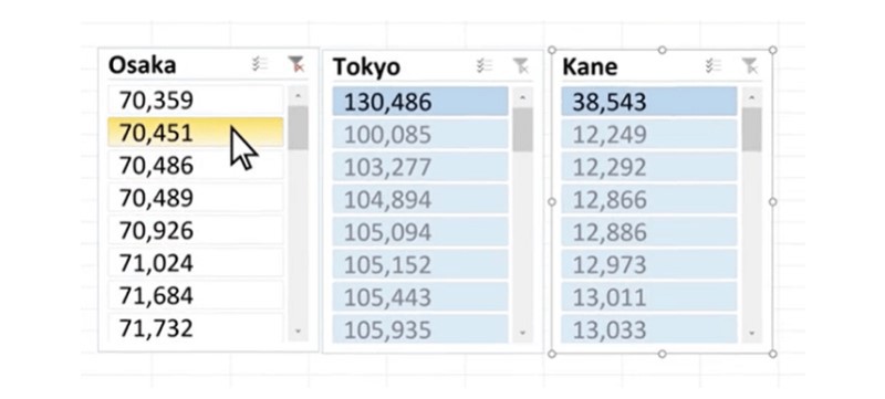
You need to filter the data by each field as follows:

To do this, you need to use the Slicer feature.
So how to use this Slicer feature? Let’s find out!

Guide to Using Slicer in Excel

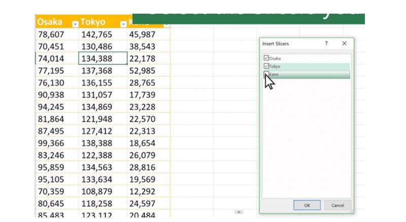
To use the Slicer feature in Excel, first select any position on the table where you want to filter the data.
Select Insert, Slicer button. Then, an Insert Slicer table appears, where you can select the field to be filtered.

For Pivot Table, under the PivotTable Tools section, select Insert Slicer to filter data.

Then, the tables containing data according to the filtered field will appear. You just need to select a data in any table, and the contents of the table or Pivot Table will change according to the selected content.

In case you have more than one Pivot Table to filter, you can connect the Slicer feature to these tables as follows:
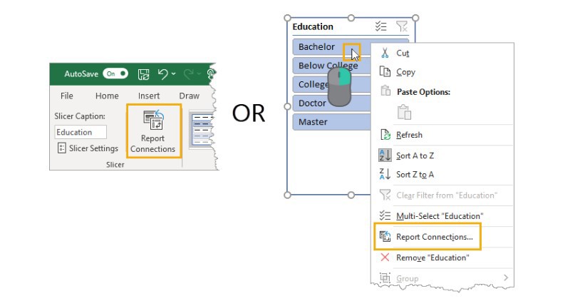
Right-click on any position in the Slicer, select Report Connections… When the Report Connections table appears, select the next Pivot Table option you want to filter.

Therefore, with a single Slicer filter, you can quickly create multiple reports.

Summary

The Slicer feature in Excel is an extremely powerful and fast data filtering tool that helps make your work much more efficient. Using it is not difficult, just practice regularly.
If you need a fully featured office software, contact Buffcom.net for support!