Updating Pivot Table Data Source Range Dynamically in Excel

Updating Pivot Table Data Source Range Dynamically in Excel. In Excel, we have various techniques like Excel Tables or Dynamic Named Ranges to dynamically change or update pivot tables. However, these methods may not be foolproof as they still require manual refreshing of the pivot table. Additionally, if you have a large dataset with thousands of rows and columns, using Excel Tables can make the file heavy and slow. In such cases, the most reliable way to automate the process is by using VBA (Visual Basic for Applications).

Updating Pivot Table Data Source Range Dynamically in Excel
Updating Pivot Table Data Source Range Dynamically in Excel
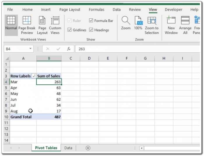
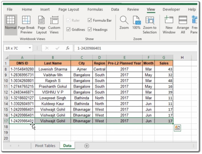
In this article, we will explore how to automatically change the data source of a pivot table and instantly reflect any new rows or columns added to the source data. To achieve this, we will utilize sheet modules and worksheet events in VBA.
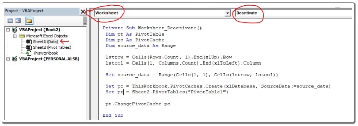
First, open the Excel file and press ALT+F11 to open the Visual Basic Editor. In the Project Explorer, locate the sheet that contains the source data and double-click on it to open its coding area.

Updating Pivot Table Data Source Range Dynamically in Excel
Within the coding area, select the worksheet from the left drop-down menu and then choose the “Deactivate” event. This will create a blank sub named “Worksheet_Deactivate”. We will place our code for dynamically changing the data source and refreshing the pivot table within this block of code. The code will run whenever you switch from the data sheet to any other sheet.
Now, let’s implement the code to update the pivot table dynamically with a new range. The code below is an example for demonstration purposes:
Private Sub Worksheet_Deactivate()
Dim pt As PivotTable
Dim pc As PivotCache
Dim source_data As Range
‘ Determine the last row and last column of the source data
lstrow = Cells(Rows.Count, 1).End(xlUp).Row
lstcol = Cells(1, Columns.Count).End(xlToLeft).Column
‘ Set the range for the source data
Set source_data = Range(Cells(1, 1), Cells(lstrow, lstcol))
‘ Create a new pivot cache with the updated source data
Set pc = ThisWorkbook.PivotCaches.Create(xlDatabase, SourceData:=source_data)
‘ Specify the pivot table to be updated (change the sheet and pivot table name as required)
Set pt = Sheet2.PivotTables(“PivotTable1”)
‘ Update the pivot table’s cache with the new source data
pt.ChangePivotCache pc
End Sub

Updating Pivot Table Data Source Range Dynamically in Excel
In this code, we utilize the “Worksheet_Deactivate” event so that the code runs to update the pivot table whenever we switch from the source data sheet. The code determines the last row and last column of the source data dynamically. It then sets the range for the source data using these values.

Updating Pivot Table Data Source Range Dynamically in Excel
A new pivot cache is created with the updated source data. The pivot table to be updated is specified (modify the sheet and pivot table name as needed), and the pivot table’s cache is updated with the new source data using the ChangePivotCache method.
By implementing this code, the pivot table will automatically update whenever there are changes in the source data. If you have multiple pivot tables using the same data source, you can use the same cache in each pivot table object.
That’s how you can dynamically change the data source range in Excel using VBA. I hope this explanation was clear. If you have any further questions, feel free to ask in the comments section below.


