Using GETPIVOTDATA Function in Excel

Using GETPIVOTDATA Function in Excel. In this article, I will guide you on how to use the GETPIVOTDATA function to retrieve summarized data from a PivotTable report, provided that the summarized data can be seen accurately and easily in the report. It is very interesting, so let’s explore it under this article!
Concept of the GETPIVOTDATA function
Returns data stored in a PivotTable report. You can use GETPIVOTDATA() to retrieve summarized data from a PivotTable report, provided that the summarized data can be seen in the report.
Syntax
GETPIVOTDATA(data_field, pivot_table, [field1, item1, field2, item2], …)
Where:
data_field: The name of the PivotTable field that contains the data you want to retrieve. This value must be enclosed in double quotation marks.
pivot_table: Refers to any cell, range of cells, or named range in a PivotTable. This information is used to determine which PivotTable contains the data you want to retrieve.
field1, item1, field2, item2, …: 1 to 126 field names and item names that describe the data you want to retrieve. The pairs can be in any order. Field names and item names that are not dates or numbers must be enclosed in quotation marks.
Activating the GETPIVOTDATA feature
The steps are as follows:
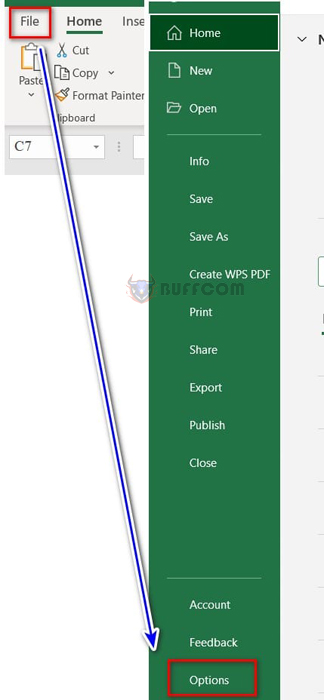
Step 1: In the Data tab, go to File => Option.
 Step 2: The Excel Options dialog box appears. Select Formulas and check the box Use GetPivotData functions for PivotTable references under the Working with formulas section.
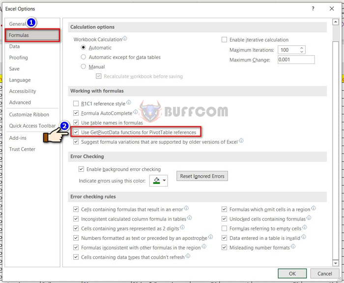 Step 3: Click OK to finish.
Example
Suppose we have a data table that summarizes sales using a PivotTable.
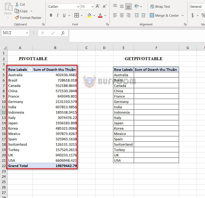 To display the accurate results when retrieving data from the PivotTable, even when the data changes constantly, you will use the GetPivotData function to retrieve data.
In the above example, we want to retrieve the Gross Sales Total value for each country to another table. You type the formula:
=GETPIVOTDATA(“Gross Sales Total”,$A$4,”Country”,”Australia”)
Or enter the equal sign and select cell B5 (the first cell in the Gross Sales Total column) to display the formula.
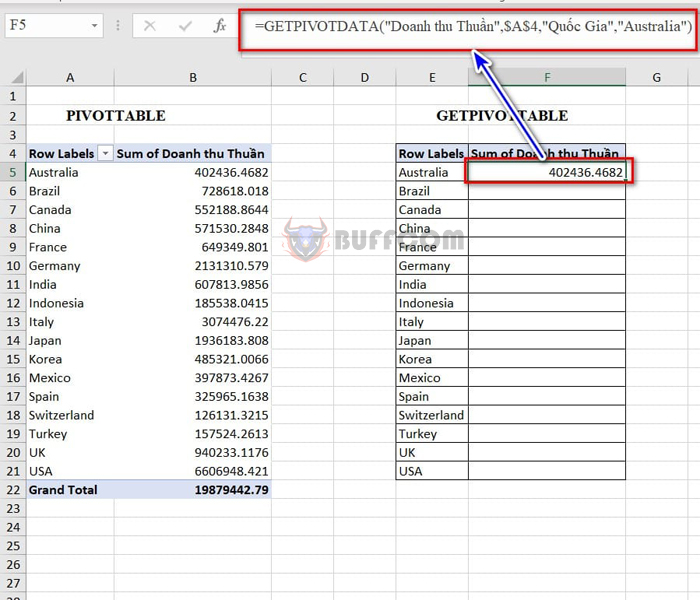 Explanation:
“Gross Sales Total”: Retrieve the value in the Gross Sales Total column.
$A$4: Starting cell of data.
“Country”: The name of the Country field you want to display the value for, and that Country is Australia.
However, the above formula only displays the result for the first cell, and you have to type another Country name for the next cell. This is time-consuming. To fix this, instead of typing the Country name, you will reference the cell containing the Country name. Specifically:
=GETPIVOTDATA(“Gross Sales Total”,$A$4,”Country”,$E5)
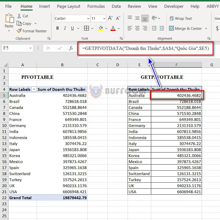 Example 2:
Revenue statistics table of each product in each country.
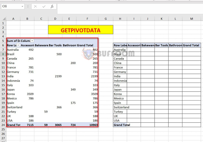 To retrieve the revenue of each product in each country from the PivotTable data to the second table, we continue to use the formula:
=GETPIVOTDATA(“Revenue”,$A$5,”Country”,$H7,”Product”,I$6)
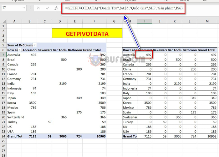 Explanation:
“Revenue”: Retrieves the displayed value from the Revenue column.
$A$5: Starting from the cell in the PivotTable which is A5.
“Country”: Name of the field that contains condition 1.
$H7: Cell that contains the first condition to be evaluated.
“Product”: Name of the field that contains condition 2.
I$6: Cell that contains the second condition to be evaluated.
That’s it, I have finished guiding you on how to use the GetPivotData function. I wish you success and don’t forget to rate my article below, with a special thanks to buffcom for the assistance!


