Using the REPT function to repeat text in Excel
Using the REPT function to repeat text in Excel: In this article, Buffcom.net will guide you on how to use the REPT function to repeat text multiple times and how to use the REPT function to create charts in Excel.
1. REPT function syntax
Function syntax: =REPT(text, number_times)
Where:
- Text: required argument, is the text you want to repeat.
- Number_times: required argument, is the number of times to repeat the text.
Note:
- If number_times is 0, the REPT function returns a blank text.
- If number_times is not an integer, the decimal part is truncated.
- If number_times is a negative number or not a number, the function returns the #VALUE! error.
- The result of the REPT function cannot exceed 32,767 characters. If it exceeds, the function returns the #VALUE! error.
2. How to use the REPT function
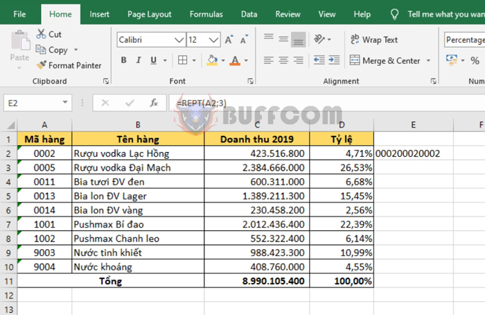
For example, we have a data table as shown in the figure below. To repeat the item code three times, the formula is as follows:
=REPT(A2,3)
Using the REPT function to repeat text in Excel
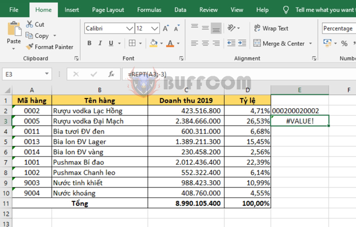
If the number_times argument is a negative number, the function will return the #VALUE! error.
=REPT(A3,-3)
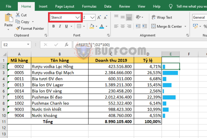
Another useful application of the REPT function is to create charts. First, select the Stencil font. Next, select the repeat character as “|” and the repeat times as a percentage multiplied by 100. The formula is as follows:
Using the REPT function to repeat text in Excel
=REPT(“|”,D2*100)
Copy the formula for the rows below, then select the highlight font color, and you will have a chart representing the proportion of items as shown in the figure below.

Therefore, this article has guided you on how to use the REPT function in Excel. Hopefully, this article will be useful to you in your work. Good luck!

