What is the VLOOKUP function? What is the function of the VLOOKUP function?
The VLOOKUP function in Excel is a basic and essential tool for every Excel user. Therefore, in this article, Buffcom.net will help you understand what the VLOOKUP function is.
The VLOOKUP function in Excel is an extremely useful tool, so anyone who uses Excel wants to learn more about this function. Don’t worry because today, Buffcom will help you understand what the VLOOKUP function is and its function. Rest assured that learning to use this function is much easier than you think!
What is the VLOOKUP function?
Basically, VLOOKUP allows you to search for a specific piece of information in a worksheet. For example, if you have a list of products with prices, you can look up the price of a particular product in the list.
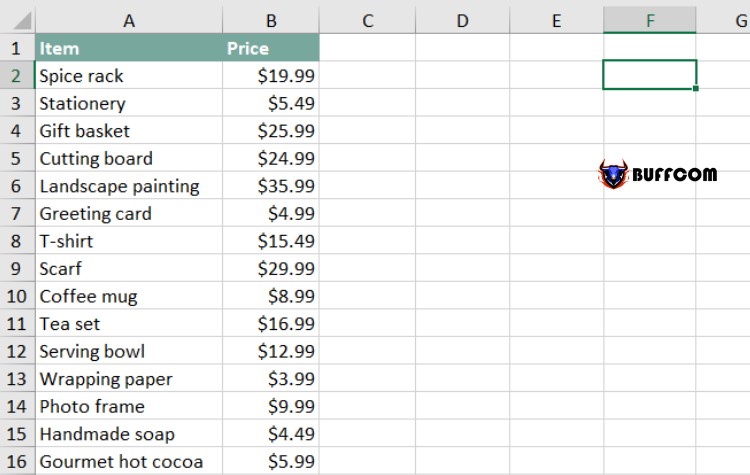
We will use the VLOOKUP function to find the price of the Photo frame product in the worksheet below. You may have already seen that its price is $9.99, but this is just a simple example. Once you have learned how to use VLOOKUP, you can apply it to much larger and more complex worksheets, and that’s when it will become really useful.
What is the VLOOKUP function? What is the function of the VLOOKUP function?
We will add the formula to cell F2, but you can add the formula to any empty cell. Any formula must start with an equal sign (=), then type the name of the formula. Our argument will need to be enclosed in parentheses, so we need to type a left parenthesis. Now it will look like this:
=VLOOKUP(
Add arguments
Now we will add our arguments. The arguments will tell VLOOKUP what to look for and where to look for it.
The first argument is the name of what you are looking for, in this case, Photo frame. Because the argument here is text, we need to enclose it in double quotes:
=VLOOKUP(“Photo frame”
The second argument is the range of cells containing the data. In this example, our data is in the range A2:B16. Just like other functions, you need to use commas to separate each argument:
=VLOOKUP(“Photo frame”, A2:B16
The important thing to know is that the VLOOKUP function will always search the first column in this data range. In this example, it will search for “Photo frame” in column A. The value returned (in this case, the price) will always need to be located to the right of that column.
The third argument is the column index number. This may sound complicated, but it’s not too bad: the first column in the data range is 1, the second column is 2, and so on. In this case, we need to find the price of the product, which is in column 2. This means our third argument is 2:
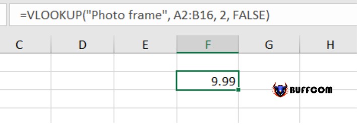
=VLOOKUP(“Photo frame”, A2:B16, 2, FALSE)
The fourth argument serves to ensure that VLOOKUP searches for an approximate match, and can be either TRUE or FALSE. If it is TRUE, it will search for an approximate match. Typically, this is only useful when the first column contains sorted numerical values. Since we are only looking for an exact match, the fourth argument should be FALSE. This is the last argument, so let’s close the parentheses:
=VLOOKUP(“Photo frame”, A2:B16, 2, FALSE)
That’s it! When you press Enter, it will return the result of 9.99.
What is the VLOOKUP function? What is the function of the VLOOKUP function?
How the VLOOKUP function works
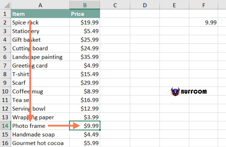
Let’s take a look at how this formula works. First, it will search the first column in a straight line from top to bottom (VLOOKUP stands for Vertical lookup). When it finds “Photo frame,” it will move to the second column to find the price. As mentioned above, the price needs to be located to the right of the product name. VLOOKUP cannot find a value located to the left of the column it is searching.
What is the VLOOKUP function? What is the function of the VLOOKUP function?
If we want to find the price of a different product, we just need to change the first argument:
=VLOOKUP(“T-shirt”, A2:B16, 2, FALSE)
Or:
=VLOOKUP(“Gift basket”, A2:B16, 2, FALSE)
However, manually adjusting the VLOOKUP formula every time we want to find the price of a different product can be very tedious. In the next example, we will explain how to use a reference cell.
Another example
Are you ready to look at a slightly more advanced example? We’ll make some changes to the spreadsheet to make it look more realistic.
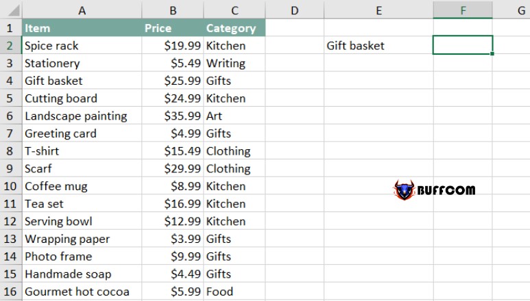
In the previous example, we typed the product name directly into the VLOOKUP formula. But in reality, you need to use a reference cell. In this example, we will type the product name into cell E2, and then our VLOOKUP formula can use the reference cell to find information about that product. Then, we just need to type a new product name into cell E2 to find any product we want.
We’ve also added a third column with the category of goods. Doing so will give us the option to search by price or product type. Now our spreadsheet will look like this:
What is the VLOOKUP function? What is the function of the VLOOKUP function?
Our formula will be similar to the previous example, but we will need to change the first three arguments. Let’s start by changing the first argument to a reference cell (make sure you delete the double quotes).
=VLOOKUP(E2, A2:B16, 2, FALSE)
To find the product category, we need to change the second and third arguments. First, we’ll change the data range to A2:C16 to include the third column. Next, we’ll change the column index number to 3 because our product category is in the third column:
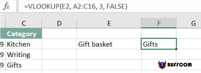
=VLOOKUP(E2, A2:C16, 3, FALSE)
When you press Enter, you will see that the product Gift basket is located in the Gifts category.
What is the VLOOKUP function? What is the function of the VLOOKUP function?
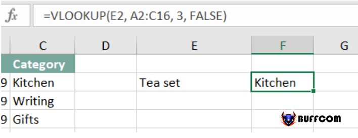
If you want to find the category of a different product, just change the data in cell E2:
What is the VLOOKUP function? What is the function of the VLOOKUP function?
Now you know what the VLOOKUP function is and how to use it in different situations. If you have any questions or suggestions, please leave a comment below for Buffcom.net to know.


