4 tips for refreshing Excel PivotTable objects

PivotTable objects rely on the underlying data, which can change frequently. If you use pivot tables in a dashboard or if it’s crucial to have up-to-date information, it’s important to refresh them regularly. In this article, we will discuss four tips to make the refresh process easy and flexible.
4 tips for refreshing Excel PivotTable objects
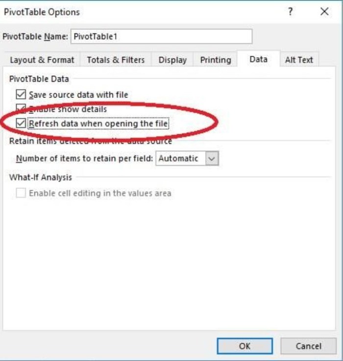
Refresh when opening the workbook:
To ensure that viewers always see the most recent data, you can set Excel to update the pivot tables automatically when you open the file. Right-click on any pivot table, choose “PivotTable Options,” go to the Data tab, and check the “Refresh data when opening the file” option.
4 tips for refreshing Excel PivotTable objects
Refresh at intervals:
If your data is critical or if the pivot table is part of a dashboard, you may need to refresh it frequently. 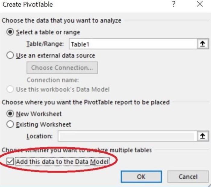 Excel allows you to set intervals for automatic refresh. To enable this feature, create the pivot table with the “Add this data to the Data Model” option checked.
 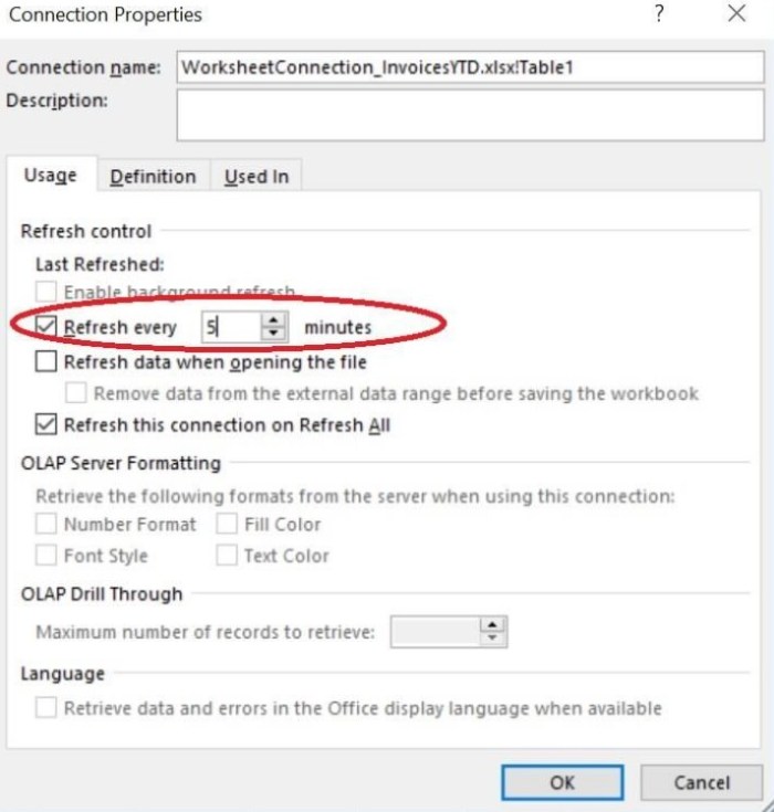 Then, go to the Analyze tab, choose “Connection Properties” from the Change Data Source dropdown, and set the refresh interval in minutes.
Preserve cell formatting:
When you add direct formatting, such as bolding headings or applying fill color, to a pivot table, it can be frustrating to see it disappear after refreshing. To preserve cell formatting, right-click on the pivot table, go to PivotTable Options, navigate to the Layout & Format tab, and check the “Preserve cell formatting on update” option.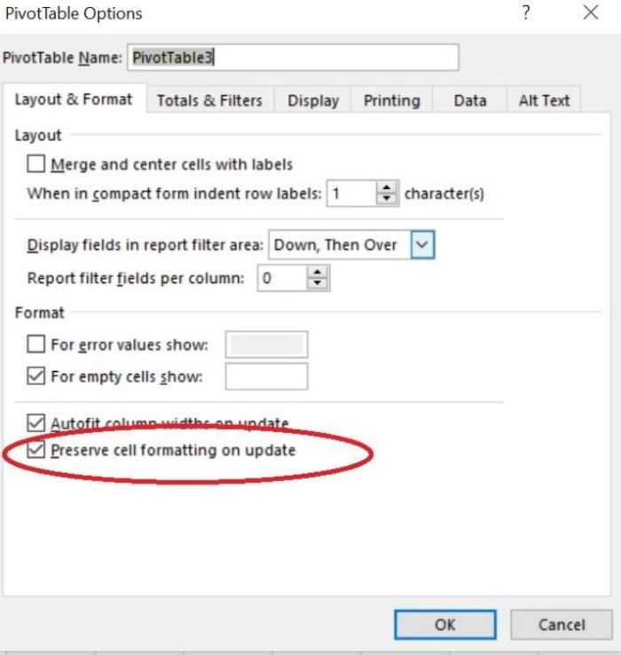
Disable AutoFit:
By default, pivot tables use autofit column widths, which can reset your custom column widths when refreshing. To prevent this, right-click inside the pivot table, go to the Layout & Format tab, and uncheck the “Autofit column widths on update” option.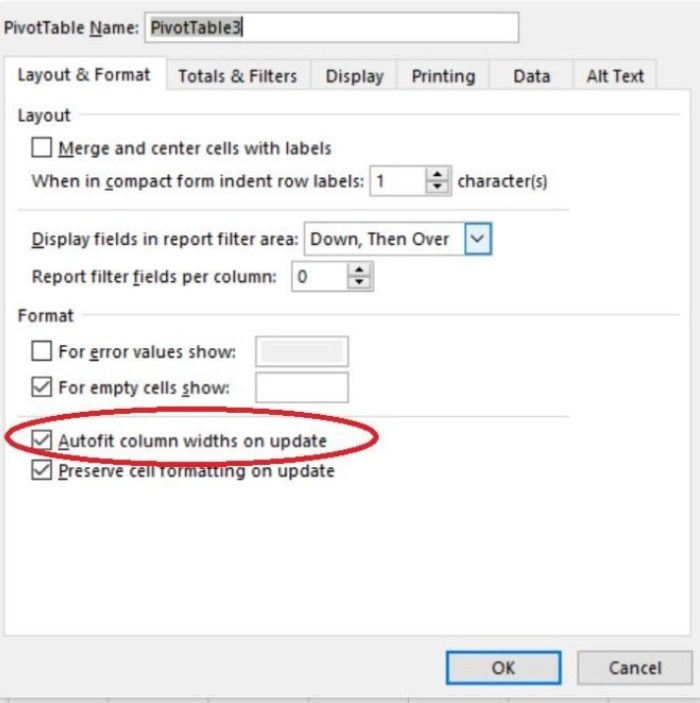
By following these tips, you can ensure that your Excel PivotTable objects are always updated, while preserving formatting and customization.


