Using the LET Function in Excel

Using the LET Function in Excel. If you work with lengthy formulas in Excel, then you’re probably familiar with the idea of named ranges to make complex formulas more readable. Now, Microsoft is taking it a step further and allowing you to name calculations and values directly within a formula. If your formula uses the same expression multiple times, you can have Excel calculate it only once, store the result within the formula, and reuse it as needed. In this article, I’ll introduce you to the LET function, which will help you overcome these challenges. Let’s find out together!

Meaning of using the LET function

The LET function in Excel allows you to name the result of a calculation and define variables within the formula, making the formula look clearer and faster to operate.

Syntax of the LET function

LET (name1, name_value1, [name2], [name_value2], …, calculation)
Where:
name1 (required) – the first name to assign. It must start with a letter.
Name_value1 (required) – the value or calculation assigned to name1.
Name2 / name_value2 (optional) – the second name and value.
Calculation (required) – a calculation using the specified names and values.

Note:
The function can handle up to 126 name/value pairs.
The last argument must be a calculation that returns a result.
Valid variable names can be used in the Name Manager. For example, “a” is valid, but “c” is not because it conflicts with R1C1-style references.

Basic formula of the LET function

If you’re not familiar with the function, an example of the simplest LET formula will help you focus on what’s necessary.
Example 1:
At cell A1, we assign the value “x”, then we enter the value of x and enter the calculation to return the result.
=LET(x,1,x+1)

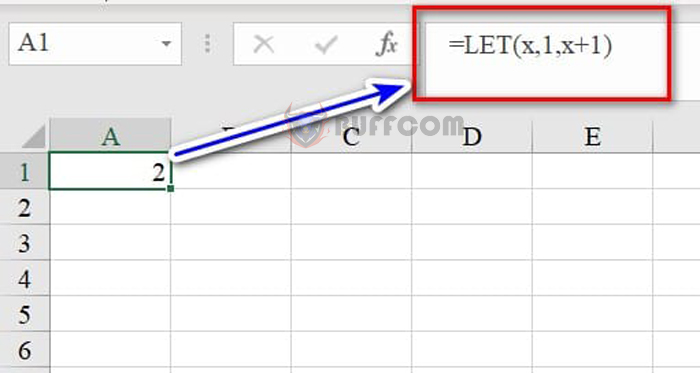In addition, instead of values, variables can be assigned to cell references.
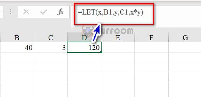
Example 2: Assign x to B1 and y to C1, we get as follows:
=LET(x,B1,y,C1,x*y)

Benefits of the LET function

Why use the LET function in Excel? The LET function can make your formula easier to read. Let’s look at an interesting example.

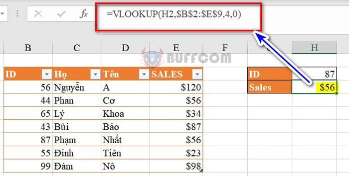
1. The VLOOKUP function below returns the sales of ID 87.
At cell H3, we enter the formula as follows: =VLOOKUP(H2,$B$2:$E$9,4,0)
Explanation: H2 is the lookup value here is 87.
$B$2:$E$9: is the lookup data range.
4: is the position of the SALES column in the data range to return.

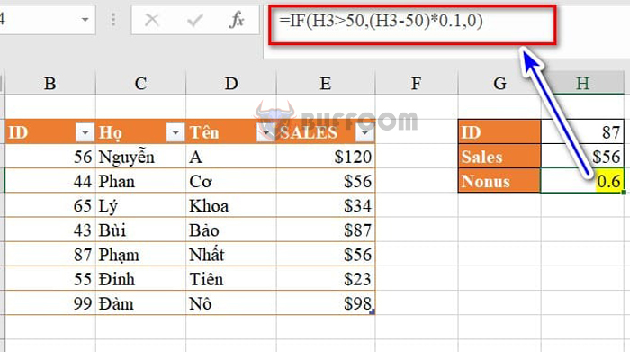
2. The formula below calculates a bonus (10% of every dollar over $50) using the IF function.
In cell H4, we enter the following formula: =IF(H3>50,(H3-50)*0.1,0)
Explanation: H3 is the cell used to compare the condition.
Alternatively, you can use the VLOOKUP function to replace H3:
In cell H4, we enter the following formula: =IF(VLOOKUP(H2,$B$2:$E$9,4,0)>50,(VLOOKUP(H2,B2:E9,4,0)-50)*0.1,0)

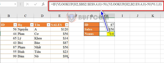This IF formula is quite difficult to read and very cluttered. But you can easily read it by using the LET function.
3. The LET function below declares the variable Sales and assigns the calculated result!
In cell H3, we enter the following formula: =LET(SALES,VLOOKUP($H2,$B$3:$E$9,4,FALSE),IF(SALES>50,(SALES-50)*0.1,0))
Explanation: SALES is the name assigned to the result returned by the vlookup function. And then use the assigned name (SALES) to compare with the required condition.

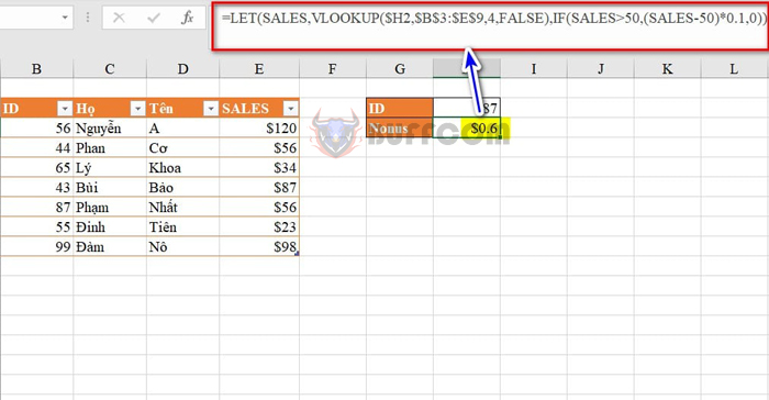So I have finished instructing you on the LET function in Excel. I wish you can perform well and don’t forget to rate Buffcom’s article!