How to use the IFERROR function in Excel

How to use the IFERROR function in Excel: During your work on Excel, if your worksheet contains too many formulas that return error values, it can be annoying. In this case, you can use the IFERROR function to fix these errors. Follow the instructions below to learn how to use the IFERROR function in Excel.
1. IFERROR function syntax
Function syntax: =IFERROR(value, value_if_error)
Where:
- Value: a required argument, is the value to check for errors.
- Value_if_error: a required argument, is the value to return if the formula in the Value argument returns an error. The following error types are evaluated: #N/A, #VALUE!, #REF!, #DIV/0!, #NUM!, #NAME?, or #NULL!.
Note: The IFERROR function in Excel takes two values (or expressions) and checks them. If:
- The first value provided does not evaluate to an error, the result returned will be that value.
- The first value provided evaluates to an error, the result returned is the second value provided.
2. How to use the IFERROR function
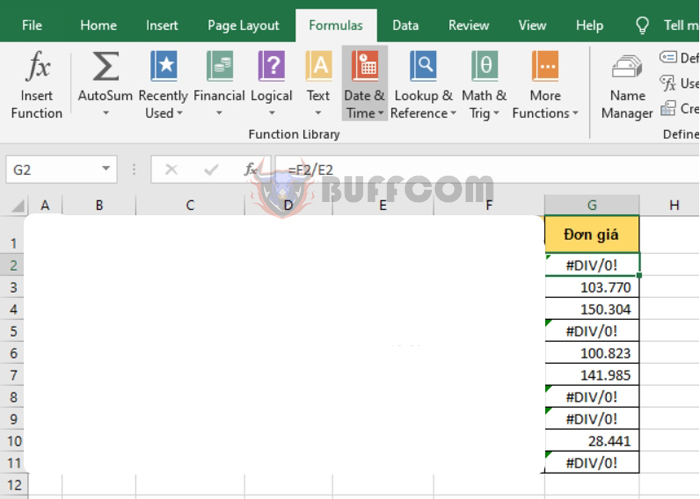
For example, consider the following worksheet. The Quantity and Total columns are given. We need to divide Total by Quantity to get the Unit Price. At this point, some products have a price error because the quantity is a denominator equals to 0, so the calculation cannot be performed. In this case, if we don’t want to display the #DIV/0! error, we can use the IFERROR function to set the return value to 0 if the formula has an error.

How to use the IFERROR function in Excel
Using the above function syntax, we can create the following formula in this case:
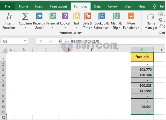
=IFERROR(F2/E2, 0)
Copying the formula for the remaining cells, we get the result:

How to use the IFERROR function in Excel
Thus, this article has instructed you on how to use the IFERROR function in Excel. Hopefully, through this article, you have learned how to use this function. Good luck!

