How to use the CUMPRINC function to calculate cumulative principal payments for a loan in Excel

How to use the CUMPRINC function to calculate cumulative principal payments for a loan in Excel: The CUMPRINC function is one of the common financial functions in Excel. The CUMPRINC function is typically used to calculate the cumulative principal payments for a loan from the first period to the last period. In this article, Buffcom.net will introduce how to use the CUMPRINC function in Excel.
1. CUMPRINC function syntax
Function syntax: =CUMPRINC(rate; nper; pv; start_period; end_period; type)
Where:
- Rate: required argument, which is the interest rate of the loan.
- Nper: required argument, which is the total number of payment periods.
- Pv: required argument, which is the present value of the loan.
- Start_period: required argument, which is the first payment period. The payment periods are numbered starting from 1.
- End_period: required argument, which is the last payment period.
- Type: required argument, which is the payment type.
Note:
- If Type is 0, it means the payment is due at the end of the period. If it’s 1, it means the payment is due at the beginning of the period.
- If Type is any number other than 0 or 1, the CUMPRINC function returns the #NUM! error value.
- If rate ≤ 0, nper ≤ 0 or pv ≤ 0, the CUMPRINC function returns the #NUM! error value.
- Rate and nper must be expressed in consistent units.
- If start_period < 1, end_period < 1, or start_period > end_period, the CUMPRINC function returns the #NUM! error value.
2. How to use the CUMPRINC function
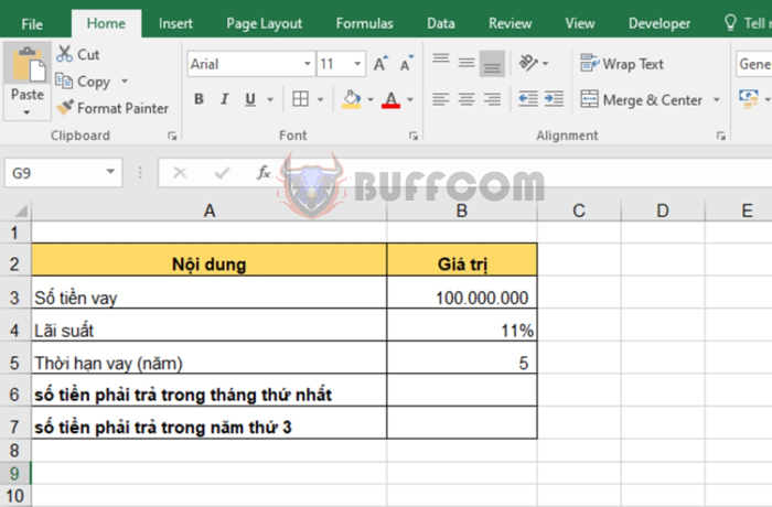
For example, if you borrow 100 million VND at an 11% interest rate for 5 years, you need to calculate the amount you have to pay in the first month and the amount you have to pay in the third year.

How to use the CUMPRINC function to calculate cumulative principal payments for a loan in Excel
a. Calculate the amount you have to pay in the first month
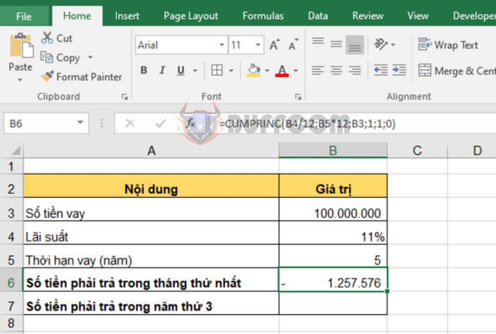
Applying the function syntax above, we have the formula to calculate the amount you have to pay in the first month as follows:
=CUMPRINC(B4/12;B5*12;B3;1;1;0)
In the above function, because we need to calculate the amount you have to pay in the first month, the units for Rate and Nper must be months. Since the interest rate is 11%/year, the monthly interest rate will be 11%/12. The number of payment periods is 5 years, which corresponds to 60 months.
 b. Calculate the amount you have to pay in the third year
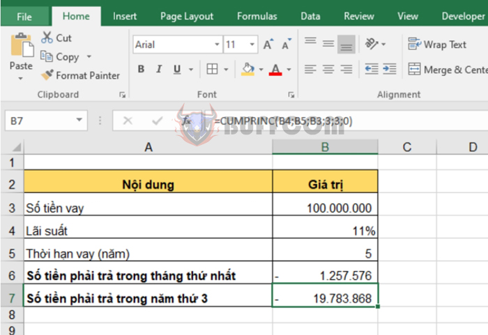
Applying the function syntax above, we have the formula to calculate the amount you have to pay in the third year as follows:
=CUMPRINC(B4;B5;B3;3;3;0)
Since the units for this calculation are years, we keep the Rate and Nper arguments the same.
 Therefore, this article has introduced how to use the CUMPRINC function in Excel. Hopefully, it will be useful to you in your work. Good luck!


