A great tip for formatting currency units in Excel
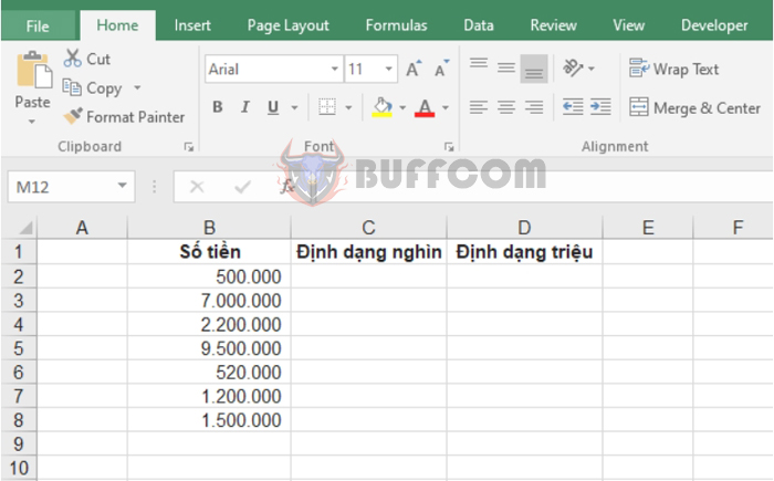
A great tip for formatting currency units in Excel: Do you not want to see many zeros after your currency amount? Instead, do you want your currency to be displayed as K, M, or thousands, millions…? Follow the steps below to learn how to format currency in Excel.
For example, let’s say you have the following currency amounts. Now, to format those amounts, follow these steps:
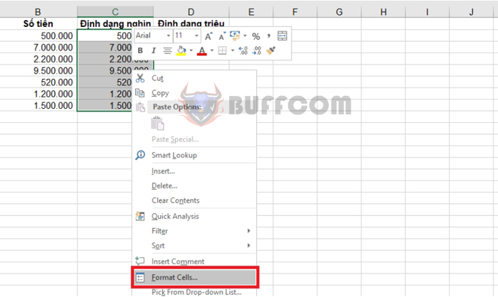
Step 1: Highlight the entire cell containing the currency amount you want to format. Then right-click and select Format Cell… Or you can use the shortcut Ctrl + 1 to quickly open the Format Cells dialog box.
A great tip for formatting currency units in Excel
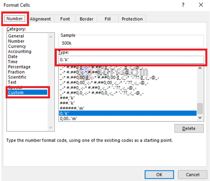
Step 2: The Format Cells dialog box appears. Select the Number tab => choose the Custom category. Here, enter 0.”k” in the Type field if you want to format three zeros in thousands as “k“. Then click OK to complete the setup.
A great tip for formatting currency units in Excel
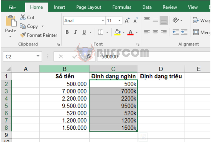
The result is that the three zeros in thousands have been converted to “k”.
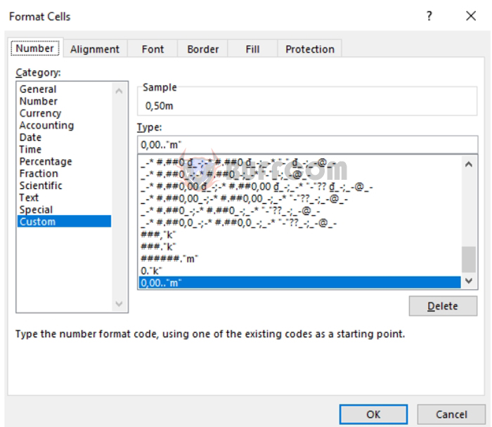
 Do the same for formatting millions. Enter 0,00..”m” in the Type field.
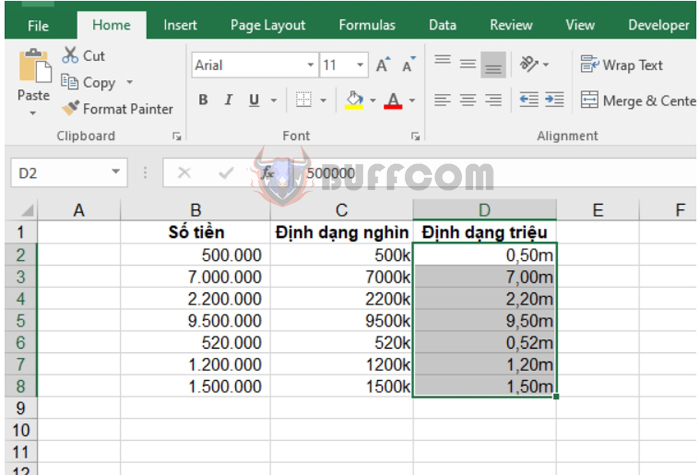
 The result is that the formatted currency amount is in millions with “m”.
 You can also customize the representation character for thousands and millions. For example, with the formula 0.” and 0,00..”, the zeros will be replaced with the words ” and ”
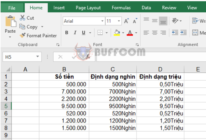 Therefore, the above article has introduced you to the tip of formatting currency in Excel. Hopefully, the article will be useful to you in using Excel. Wish you success!

