How to use the FV function to calculate the future value of an investment in Excel
How to use the FV function to calculate the future value of an investment in Excel: The FV function calculates the value at a future date that investors will receive when they make a single or multiple periodic investments with a constant interest rate. For example, if you plan to save a certain amount of money over a period of 10 years and want to calculate how much you will have in your account after that time, you can use the FV function. This article will guide you on how to use the FV function in Excel.
1. Syntax of the FV function
Function syntax: =FV(rate, nper, pmt, [pv], [type])
Where:
- Rate: Required argument, the interest rate per period (monthly, quarterly, yearly).
- Nper: Required argument, the total number of payment periods.
- Pmt: Required argument, the payment made in each period. This amount is fixed. Usually, pmt includes both principal and interest but does not include any fees.
- Pv: Optional argument, the present value or initial investment amount. If pv is omitted, it is assumed to be 0.
- Type: Optional argument. Either 0 or 1 to indicate the timing of the payment. 1 if the payment is made at the beginning of the period, 0 if the payment is made at the end of the period. If the type argument is omitted, it is assumed to be 0.
2, How to use the FV function
Example: You want to save a certain amount of money over a period of 10 years. Initially, you deposit 100 million into a savings account with an interest rate of 5% per year. Each subsequent year, you deposit an additional 50 million into the account. Calculate how much money you will have in your account at the end of 10 years.
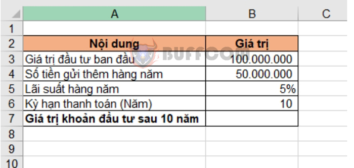
In this case, two scenarios can occur:
- The initial deposit amount from the previous period and the additional deposits start from the next period. In this case, Type = 0 (next period is the end of the previous period).
- The initial deposit amount from the previous period and the additional deposits are made in the same first year as the principal. In this case, Type = 1.
Scenario 1: The initial deposit amount from the previous period and the additional deposits start from the next period
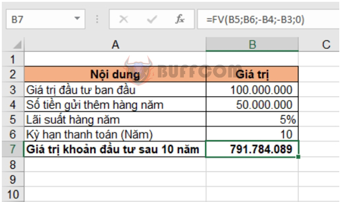
In this scenario, the Type argument is set to 0. The formula to calculate the investment value after 10 years is as follows:
=FV(B5, B6, -B4, -B3, 0)
Where:
- B5 is the interest rate (5%).
- B6 is the number of payment periods (10 years).
- -B4 is the annual deposit amount.
- -B3 is the initial deposit amount.
- 0 indicates that the additional deposits start from the next period.
 Scenario 2: The initial deposit amount from the previous period and the additional deposits are made in the same first year as the principal
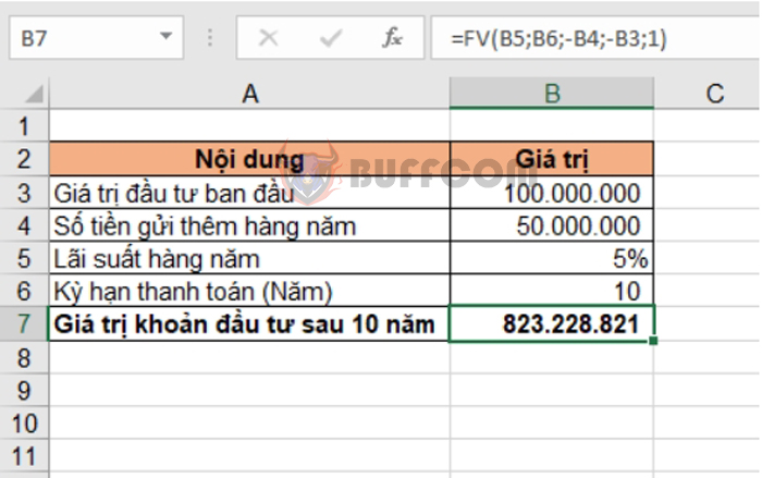
In this scenario, the Type argument is set to 1. The formula to calculate the investment value after 10 years is as follows:
=FV(B5, B6, -B4, -B3, 1)
Where:
- B5 is the interest rate (5%).
- B6 is the number of payment periods (10 years).
- -B4 is the annual deposit amount.
- -B3 is the initial deposit amount.
- 1 indicates that the additional deposits are made in the same first year as the principal.
How to use the FV function to calculate the future value of an investment in Excel
That’s it! The above article has guided you on how to use the FV function in Excel. Good luck with your Excel tasks!


