How to Use the PMT Function to Calculate Periodic Loan Payments in Excel

How to Use the PMT Function to Calculate Periodic Loan Payments in ExcelThe PMT function is a financial function commonly used to calculate the periodic payments of a loan with a fixed interest rate. This article will guide you on how to use the PMT function to calculate periodic loan payments in Excel.

PMT Function Syntax
The syntax of the PMT function is as follows: =PMT(rate, nper, pv, [fv], [type])
Where:

• Rate: Required argument. This is the periodic interest rate of the loan.
• Nper: Required argument. This is the total number of payment periods for the loan.
• Pv: Required argument. This is the present value of the loan (the principal).
• Fv: Optional argument. This is the future value (or remaining balance) of the loan after the final payment. If omitted, it is assumed to be 0, indicating the loan will be fully paid off.
• Type: Optional argument. Choose between the value 0 or 1. If Type is omitted, it is assumed to be 0, representing payments made at the end of each period, and 1 represents payments made at the beginning of each period.

Note:

• The payment amount returned by the PMT function includes both principal and interest but does not include any fees, charges, or taxes that may accompany the loan.
• Rate and Nper must be consistent in terms of the same time value.
• If Nper is required in months but the interest rate given in the problem is per year, you need to convert the rate to a monthly rate.

2. Using the PMT Function

a. Using the PMT function to calculate periodic loan payments
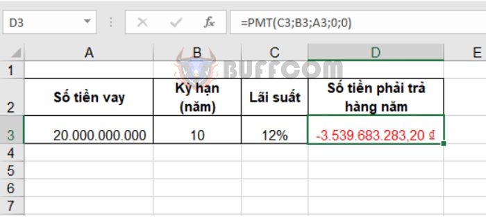
Let’s assume you borrow a loan of 20 billion VND with a 5-year term and an interest rate of 12% per year. Calculate the annual loan payment amount.

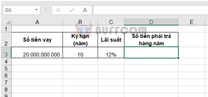
To calculate the annual payment amount, enter the formula in cell D3: =PMT(C3, B3, A3, 0, 0)

The result will be the annual payment amount of 3,539,683,283.2 VND, as shown in the example below:

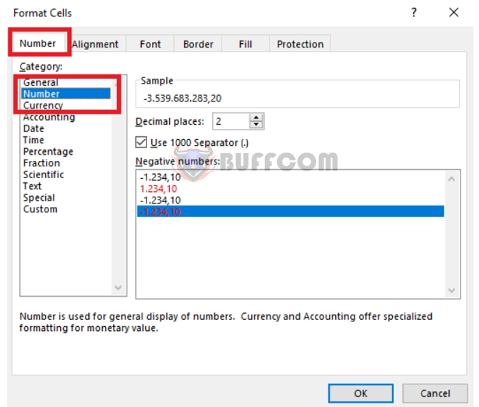
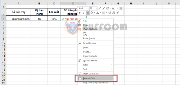
The default result of the PMT function will be in currency format. If you do not want to use this format, you can change the number format by right-clicking and selecting “Format Cells…” or by pressing the Ctrl + 1 key combination to open the Format Cells dialog box.

In the current Format Cells dialog box, select the Number tab and choose the Number category. Then, you can adjust the desired number formats here.

b. Using the PMT function to calculate savings contributions to reach a goal
Let’s say you set a goal to make monthly savings deposits for 6 months. The desired amount to accumulate after 6 months is 1 billion VND, and the savings interest rate is 1% per month.

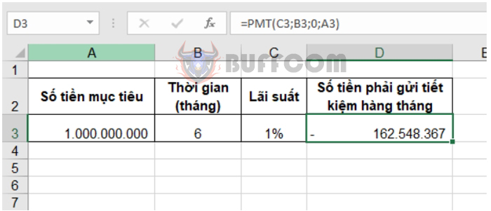
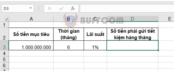To calculate the monthly savings deposit amount, use the formula in cell D3: =PMT(C3, B3, 0, A3)

The result will be a monthly deposit amount of 162,548,367 VND, so that after 6 months, you will accumulate 1 billion VND.

That’s it! This article has guided you on how to use the PMT function to calculate periodic loan payments in Excel. Good luck with your calculations!