How to limit columns in a filtered result set in Microsoft Excel

When using Microsoft Excel‘s Advanced Filter feature, you have the ability to display records that match specific criteria. Additionally, you can control the number of columns returned by this feature.
While it’s easy to filter records in Excel and view entire records that meet the specified criteria, you might be interested in limiting the columns in the filtered result set. Unfortunately, this cannot be achieved through a simple Excel filter, as it filters the source data in place.
However, by utilizing the advanced filter functionality, you can filter both the records and the columns. In the following steps, I’ll demonstrate how to use Excel’s Advanced Filter feature to obtain a filtered set based on two criteria columns, and then how to restrict the filtered set to only those two columns.
Please note that I’m using Microsoft 365 desktop on a Windows 10 64-bit system, but these steps can be applied to earlier versions as well.
Understanding Microsoft Excel’s Advanced Filter
The Advanced Filter feature in Excel does not rely on a dropdown list of filtering options and values. Instead, you enter criteria at the sheet level, and the feature either filters the source data or copies a filtered set to another location.
This feature involves three components:
- Source data: The data you wish to filter.
- Criteria: The values that should match the source data.
Location: Determines whether to filter in place or copy the filtered results to another location.
With the advanced filter in Excel, you can express criteria across multiple columns. While the simple Filter feature allows you to do this, it requires expressing the criteria one column at a time. Conversely, an advanced filter enables you to express criteria for all columns in the dataset simultaneously. Moreover, you can use more complex criteria with the advanced filter.
Let’s proceed with an example to demonstrate how to apply an advanced filter to obtain all columns in a filtered result set.
How to Use Advanced Filter in Excel
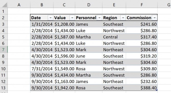
Let’s consider a quick example using a table named “Commission,” as shown in Figure A. Suppose you want to view all the records for employees whose names start with “M” and whose corresponding commission is less than $250. Additionally, you want to copy the filtered results to another location rather than filtering the source data directly.
Figure A:
[Image: Susan Harkins/TechRepublic. We’ll use an advanced filter on this data set.]
Assuming you already have the source data, let’s set up the criteria and location:
- Copy the header row to another sheet, creating two copies, as illustrated in Figure B. Although this step can be performed on the same sheet, using another sheet makes it easier.
- In cell D3 (Personnel column), enter the criteria string “M*.”
In cell F3 (Commission column), enter the criteria string “<=250.” Since both criteria expressions are in the same row, Excel treats them as an “AND” operation. The filter will return any record where the Personnel value starts with “M” and the Commission value is less than or equal to 250. To perform an “OR” operation, place one of the criteria expressions in the next row.
Figure B:
- [Image: Susan Harkins/TechRepublic. Prepare the criteria and location ranges.]
Once the criteria are set and both headers are in place, let’s run the Advanced Filter feature:
- Click on the sheet tab that contains the criteria and location headers (Figure B). In the example file, this sheet is named “Results.” The active sheet must be the location sheet.
- Go to the Data tab and click on “Advanced” in the Sort & Filter group.
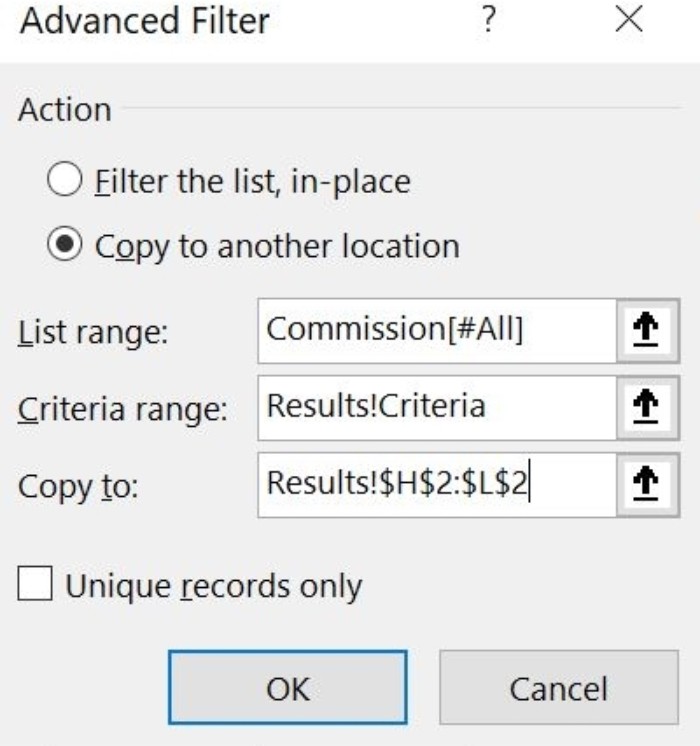
- In the resulting dialog, identify the source data, criteria, and location for the result
Figure C:

How to limit columns in a filtered result set in Microsoft Excel
[Image: Susan Harkins/TechRepublic. The advanced filter settings.]
If you’re wondering why there is no filtered result set, don’t worry, nothing went wrong. Upon careful review of the source data, you’ll notice that there isn’t a record that meets the specified criteria!
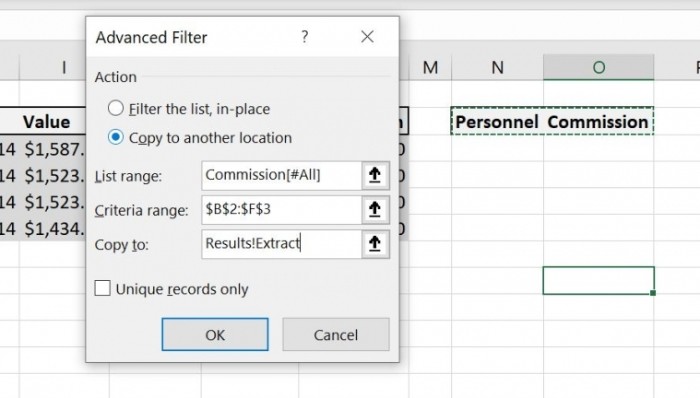
Let’s make a slight change to the criteria and observe the outcome. Modify the equality operator in cell F3 from “<=” to “>=” and run the filter again. Excel will display a warning that the destination range is not large enough. Click “Yes” to proceed, as there is sufficient space for the result set. As shown in Figure D, you’ll see that there are four records that meet the revised criteria.
Figure D:

How to limit columns in a filtered result set in Microsoft Excel
[Image: Susan Harkins/TechRepublic. Four records meet the criteria expressions in C3 and E3.]
As you can see, this feature requires some initial preparation, but it’s straightforward to execute and produces impressive results. However, the resulting set still displays the full record. Now, let’s proceed to limit the columns.
How to limit the columns using Excel’s Advanced Filter
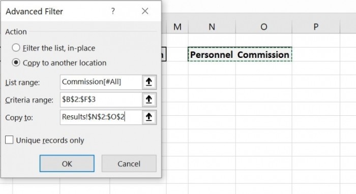
Restricting the columns returned by an advanced filter is a simple process. Just modify the header cells to correspond to the columns you wish to view. Figure E illustrates a new header row in N2:O2.
Figure E:

How to limit columns in a filtered result set in Microsoft Excel
[Image: Susan Harkins/TechRepublic. To reduce the columns, reduce the header cells.]
Perform the advanced filter as before, but this time specify N2:O2 as the “Copy to” range (Figure E). The result set, as shown in Figure F, will contain four rows and only two columns. By adjusting the header cells, you can limit the number of columns copied to the result set.
Figure F:

How to limit columns in a filtered result set in Microsoft Excel
[Image: Susan Harkins/TechRepublic. The “Copy to” range reduces the number of returned columns to two.]
Copying only the desired columns to a filtered result set is not the same as applying a filter, but it allows you to work exclusively with the data you need.


