Getting the Relative Column Index in Excel

Getting the Relative Column Index in Excel. This article provides instructions on how to obtain the relative column index in Excel. The scenario involves marking the index for data with an index column that may not start from the first column of the worksheet. To achieve this, the COLUMN function and a simple logic are utilized to determine the column index in the data.

Getting the Relative Column Index in Excel

The COLUMN function returns the column number of a given cell reference. The syntax for the function is as follows: =COLUMN([cell_reference]). If no argument is provided, the function returns the column number for the cell where the formula is used.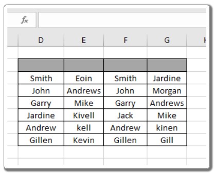

To construct the formula, a difference of 1 is created between two numbers, which are the outcomes of two COLUMN functions. The formula is then extended to the remaining columns of the data. The generic formula is as follows: =COLUMN() – COLUMN(cell_ref).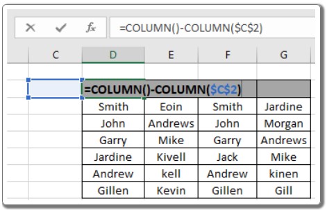

An example is provided to illustrate the usage of this function. A data table with names is used, and the goal is to mark each column with its index in the given index row.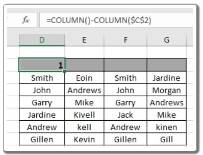

The customized formula in cell D2 is as follows: =COLUMN() – COLUMN($C$2). The COLUMN() function returns 4, the corresponding column number for the cell, while COLUMN($C$2) returns 3, the column number for column C. The dollar sign ($) is used to fix the cell reference.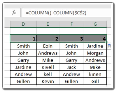

The formula is then copied to the rest of the cells using the Ctrl + R shortcut key or the drag-right feature in Excel.

In Excel 2016, there is an alternative method to achieve the same result. By dragging down the selected cells, Excel automatically extends the values. This method is demonstrated by typing numbers 1 and 2 in the first and second index spaces, selecting the cells, and dragging them right until the column index is filled.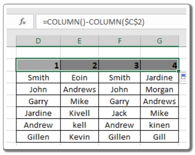

The article concludes by encouraging further exploration of Excel cell reference functions and inviting readers to provide any queries or feedback.