A very simple example of an array formula in Excel
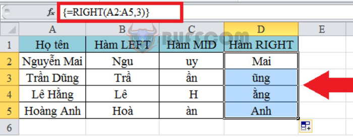
The array formula in Excel is a powerful tool for users to solve difficult problems. A simple array formula can represent multiple calculations at once and thus replace many commonly used formulas. It is strange that over 90% of users have never used array formulas in their spreadsheets because they are hesitant to start with an array formula. This article will introduce you to some extremely simple examples of array formulas in Excel. Please read on.
1. Extremely simple examples of array formulas in Excel
At the Excel interface, users need to have data tables like the one below. In this example, you need to calculate the total amount based on the unit price and quantity of some items.
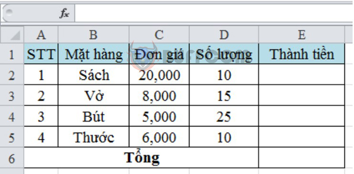
A very simple example of an array formula in Excel
Typically, users need to calculate the total amount according to the formula: =Unit price * Quantity. Then you use the SUM function to calculate them together and get the result as follows:
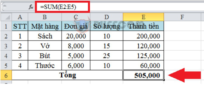
A very simple example of an array formula in Excel
Instead of doing it the above way, you can use an array formula. To do this, you enter the formula: =SUM(C2:C5*D2:D5) and then press the Ctrl + Shift + Enter key combination. Then the result returns as follows:
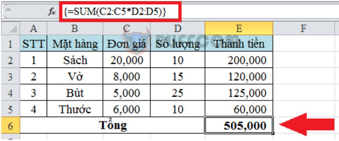
A very simple example of an array formula in Excel
With this method, you can perform calculations faster. Note that for an array formula, you need to use the Ctrl + Shift + Enter key co
mbination to end the formula. Because if the result is not returned, an error will be reported as shown below:
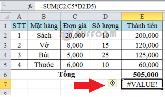
A very simple example of an array formula in Excel
2. Example of an array formula for creating a constant
To create an array constant, you need to enter a list of items. In the example below, you need to select cell A1:D1. Then enter the list of Congratulations, You, Succeeded, and put them in curly braces. Then press the Ctrl + Shift + Enter key combination to use the array formula.
By observing the method and the result image below, you will understand more clearly.

A very simple example of an array formula in Excel
3. Some other examples using array formulas
In addition to the SUM function example above, you can do the same with other functions such as LEFT, MID, RIGHT, MAX…
3.1. Array formula with LEFT, RIGHT, MID function
With these 3 functions, you can extract n characters from a string from the left, right or middle. You just need to enter the fo
rmula as usual and then press Ctrl + Shift + Enter. Then the result returns as follows:
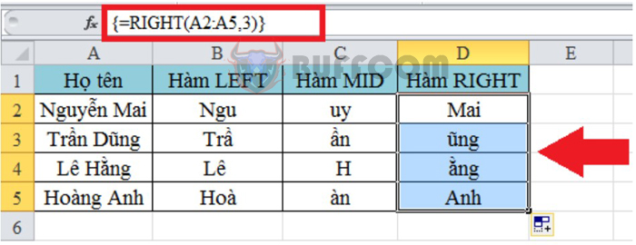
A very simple example of an array formula in Excel
3.2. Array formula with MAX function
In this example, you need to find the maximum value of A-B. Normally, you will find the A-B difference in the cells below and use the MAX function to find the maximum value. After completing the steps, the result returns as follows:
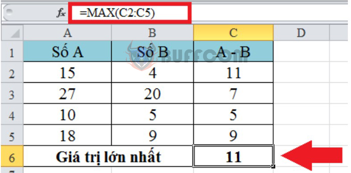
A very simple example of an array formula in Excel
Instead of having to perform the above steps, you can use array formulas to make calculations faster. Enter the formula: =MAX(A2:A5-B2:B5) and then press the keyboard combination Ctrl + Shift + Enter. By looking at the image below, you will understand better how to do it:
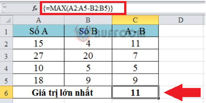
A very simple example of an array formula in Excel
The article above by Buffcom.net has introduced users to very simple examples of array formulas in Excel. Hopefully, this article will provide useful information for readers when working with Excel. Wish you success in your work!


