Automatically Color Rows and Columns Based on Mouse Pointer

Automatically Color Rows and Columns Based on Mouse Pointer. With a large spreadsheet containing many rows and columns, it can be difficult to keep track of which row and column you are currently selecting. Today, Buffcom will guide you on how to automatically color cells based on the mouse pointer, which helps prevent data entry or verification errors.
Automatically Color – Coloring Rows
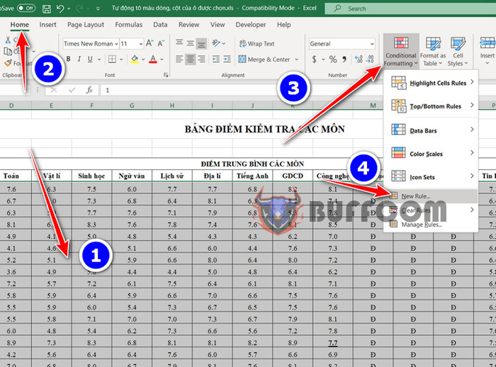
First, select the range of data and click on Home, then select Conditional Formatting -> New Rule.
Automatically Color Rows and Columns Based on Mouse Pointer
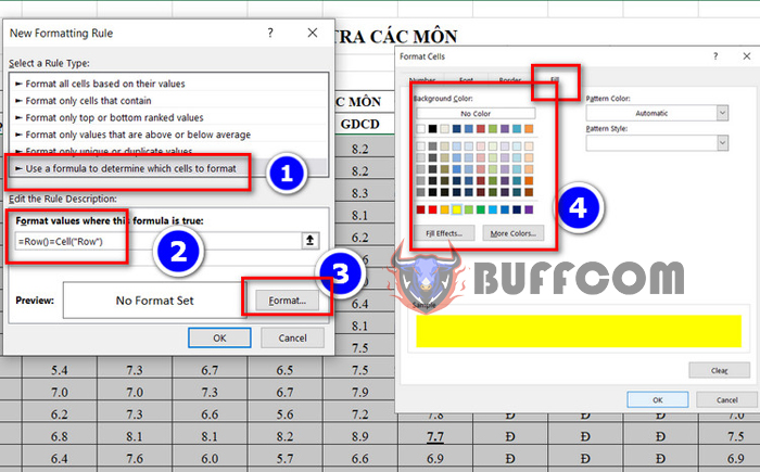
In the new window, select “Use a formula to determine which cells to format”, then enter the formula =Row()=Cell(“Row”) in the “Format values where this formula is true” box. Select the desired fill color, then click OK.
Automatically Color Rows and Columns Based on Mouse Pointer
Now, the color of the row has been applied, but it does not automatically follow the mouse pointer when you click on other rows. You can press F9 to manually refresh, but to automatically follow the mouse pointer, continue with the following steps.
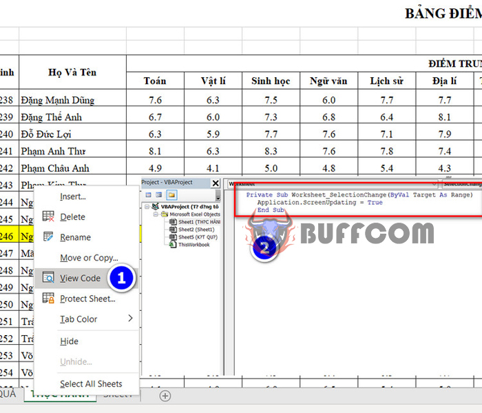
Right-click on the sheet, select “View code”, and then copy and paste the following code:
Private Sub Worksheet_SelectionChange(ByVal Target As Range)
Application.ScreenUpdating = True
End Sub
Automatically Color Rows and Columns Based on Mouse Pointer
With this code, the row where the mouse pointer is located will automatically change color.
Coloring Columns
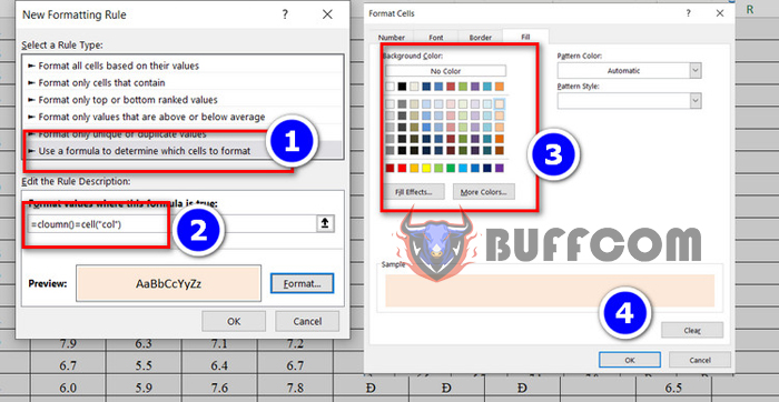
To color columns instead of rows, follow the same steps as above but replace the formula with =Column()=Cell(“col”).
Automatically Color Rows and Columns Based on Mouse Pointer
Coloring Cells
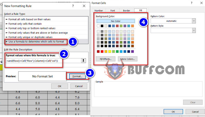
Finally, if you want to color individual cells based on the mouse pointer, use the formula =and(Row()=Cell(“Row”),Column()=Cell(“col”)) in the “Format values where this formula is true” box.
Automatically Color Rows and Columns Based on Mouse Pointer
In this way, you can easily manage and keep track of the selected cell, row, and column by the visual color changes.
Thank you for reading Buffcom‘s article. Wishing you success!

