Counting cells that are not equal to multiple criteria in Excel
Counting cells that are not equal to multiple criteria in Excel. In this article, we will learn how to count cells in Excel that do not match specific criteria. To put it simply, we want to count data based on certain conditions in an array, counting cells that do not contain certain values using Excel functions. We will use wildcard characters to match strings and perform functions accordingly.
Counting cells that are not equal to multiple criteria in Excel
There are three methods we will explore to achieve this:
Method 1: Using SUMPRODUCT, MATCH, and ISNA functions
- Use the MATCH function to identify the positions where values need to be counted, and the ISNA function to catch #NA errors.
- SUMPRODUCT then returns the sum of these values, effectively counting cells where the criteria are not met.
The formula is: = SUMPRODUCT(–(ISNA(MATCH(range, values, 0))))
Where:
- range is the array of cells to count.
- values is the array of values to be ignored in the count.
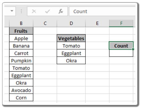
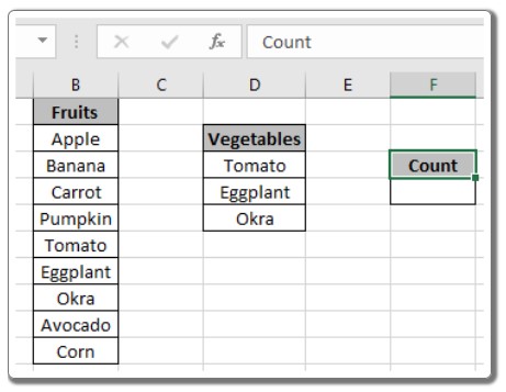
Example: Let’s consider a list of fruits in one column and vegetables in another. To count only the fruits, not considering vegetables:
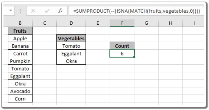
Formula: = SUMPRODUCT(–(ISNA(MATCH(fruits, vegetables, 0))))
Counting cells that are not equal to multiple criteria in Excel
Where:
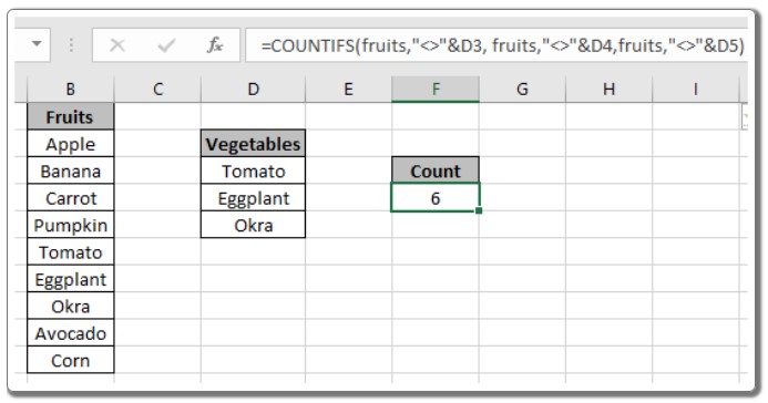
- fruits is the named range for cells B2:B10 (containing fruits).
- vegetables is the named range for cells D3:D5 (containing vegetables).
Counting cells that are not equal to multiple criteria in Excel
Method 2: Using COUNTIFS function
- The COUNTIFS function allows us to count cells that meet multiple criteria.
- We use the “<>” operator, which stands for “not equal to,” to exclude specific values from the count.
The formula is: = COUNTIFS(range, “<>” & value1, range, “<>” & value2, …)
Where:
- range is the array of cells to count.
- value1, value2, etc. are the values to be ignored in the count.
Example: Continuing with the fruits and vegetables example, to count only the fruits:
Formula: = COUNTIFS(fruits, “<>” & D3, fruits, “<>” & D4, fruits, “<>” & D5)

Counting cells that are not equal to multiple criteria in Excel
Method 3: Using COUNTA function and subtraction
- We can calculate the count of all non-empty cells in the range using the COUNTA function.
- Then, we subtract the count of cells that match specific criteria using the COUNTIF function.
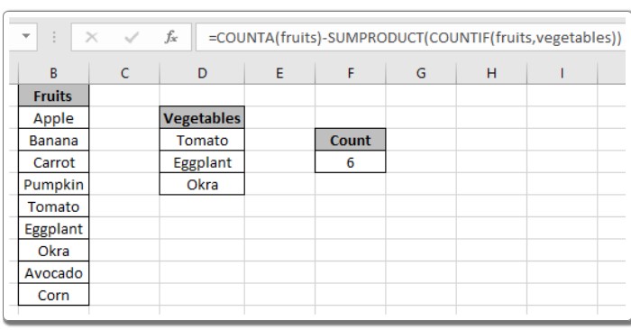
The formula is: = COUNTA(range) – SUMPRODUCT(COUNTIF(range, values))
Where:
Counting cells that are not equal to multiple criteria in Excel
- range is the array of cells to count.
- values is the array of values to be ignored in the count.
Example: For the fruits and vegetables example:
Formula: = COUNTA(fruits) – SUMPRODUCT(COUNTIF(fruits, vegetables))
These methods allow us to count cells that do not match specific criteria in Excel. You can choose the most suitable method based on your requirements. Feel free to explore more Excel count functions for further functionalities. If you have any questions or feedback, please don’t hesitate to ask.