How to Efficiently Navigate an Excel Workbook Using Named Ranges

How to Efficiently Navigate an Excel Workbook Using Named Ranges. When working with an Excel workbook, there are various methods to move around sheets or within a sheet. However, to cater to users who may be unfamiliar with Excel or to simplify navigation in a busy file, you can include shortcuts using named ranges and hyperlinks. In this article, I will demonstrate how to utilize named ranges and hyperlinks as convenient shortcuts to important data.

How to Efficiently Navigate an Excel Workbook Using Named Ranges

Creating a Named Range in Excel:

Named ranges are commonly used as references for cells or cell ranges in expressions, but they can also be used for navigation. Before using a named range to navigate, you need to create one. Follow these steps:

1. Select the desired cell or range of cells.
2. In the Name Box control, located to the left of the formula bar, enter a name for the range.
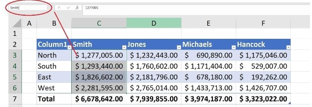
3. For example, let’s name the data in cell range C3:C6 as “Smith” (Figure A).
   

   How to Efficiently Navigate an Excel Workbook Using Named Ranges

   • Select C3:C6 (or a single cell).
   • Click inside the Name Box control, type “Smith,” and press Enter.
   • Names must start with an alphabetic character, an underscore (_), or a backslash (). They cannot start with a number or contain spaces, most punctuation characters, or conflict with a cell reference. Names are not case-sensitive.

Navigating to a Named Range using the Name Box Control:

The Name Box control also serves as a quick navigation tool. Follow these steps:

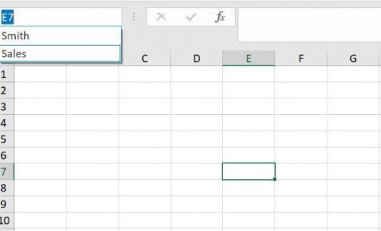
1. Click the dropdown arrow in the Name Box control.
2. Select the desired named range to navigate to that range.
3. For example, you can move to a different sheet and then select “Smith” from the dropdown (Figure B). Excel will promptly select the corresponding data on the sheet. This method also works in the browser. Alternatively, you can press F5 and choose a named range.
   

   How to Efficiently Navigate an Excel Workbook Using Named Ranges

Creating Hyperlinks to Navigate to Named Ranges:

While the Name Box control requires users to have knowledge of its functionality, in situations like dashboards, it’s beneficial to provide intuitive navigation tools such as hyperlinks. You can create a hyperlink that directs users to a named range. Here’s how:

How to Efficiently Navigate an Excel Workbook Using Named Ranges

1. Right-click the cell containing the desired text value (e.g., “Smith”) and select “Link” from the submenu.
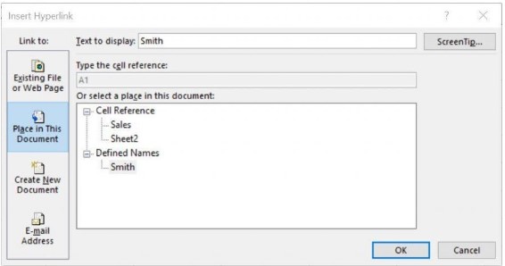
2. In the resulting dialog, choose “Place In This Document” in the left pane.
3. Select the named range (“Smith” in our example) from the Defined Names list (Figure D) and click “OK.”
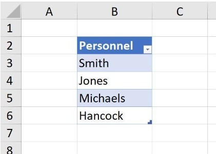
4. The resulting hyperlink will appear (Figure E). Users can click on it (e.g., “Smith” in cell B3) to access the sales data associated with that named range.

These hyperlinks are user-friendly and familiar, making them intuitive for viewers and users. You can also assign hyperlinks to graphics. To remove a hyperlink, simply right-click on it and select “Remove Hyperlink” from the submenu.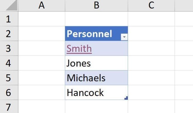

By creating named ranges and incorporating them into navigation shortcuts, you can enhance the user experience and simplify data access. If you have other methods of using named ranges for shortcuts, feel free to share them in the discussion accompanying this article.