Finding the Lowest Value in a List of Numbers (N)
To find the lowest values in Excel from a list of numbers, you can utilize the SMALL function. This function allows you to retrieve not only the smallest value, but also the 2nd, 3rd, 4th, or any Kth smallest value from the list.
Finding the Lowest Value in a List of Numbers (N)
In this tutorial, we will demonstrate how to write a formula using this function.
Excel Formula to Obtain the Lowest Number
Follow the steps below:
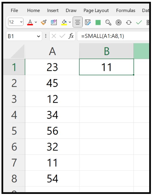
- Enter the SMALL function in a cell.
- In the first argument (array), refer to the range where the list of numbers is located.
- In the second argument (k), input 1 since you want to obtain the 1st lowest number from the list.
- Press Enter to obtain the result.
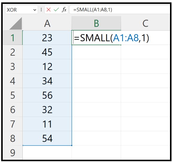
Upon pressing Enter, it will return 11 as the result, which is the lowest number in the specified range.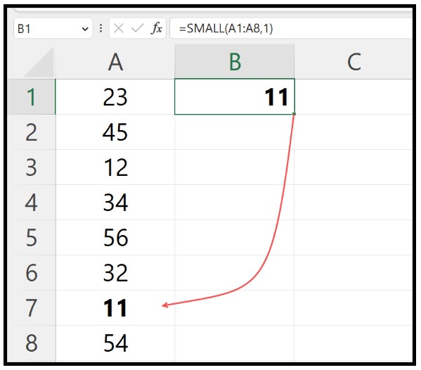
Finding the Nth Lowest Values from a List of Numbers
If you wish to retrieve the Nth smallest value from the same list, you only need to modify the value in the second argument (k) of the function. For instance, if you want to obtain the 3rd smallest value, the formula would be: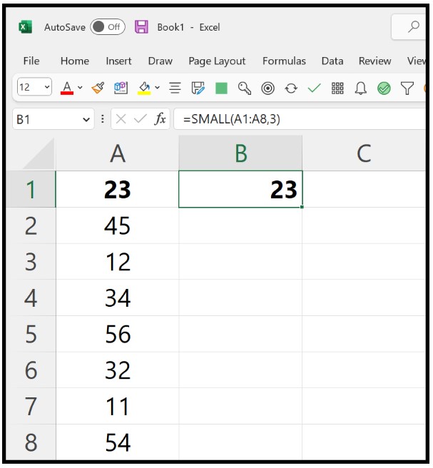
=SMALL(A1:A8,3)
This formula will return 23, which is the 3rd lowest number in the list.
Finding the Lowest 3 Values
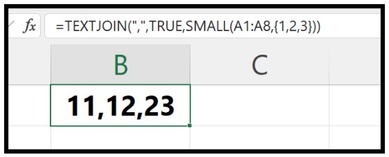
Suppose you need to obtain the lowest three values within a single cell. To achieve this, you can combine the TEXTJOIN function with the SMALL function, as demonstrated in the example below: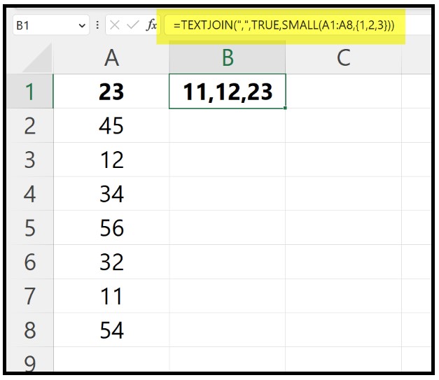
=TEXTJOIN(“,”,TRUE,SMALL(A1:A8,{1,2,3}))
Within the SMALL function, we have used {1,2,3} as the argument for k in order to obtain the 3 lowest values from the list.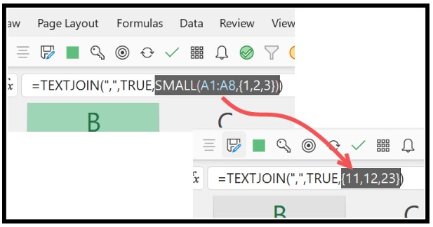
This formula will return 11, 12, and 23, as they are the 3 lowest numbers in the list. If you want these three numbers to appear in a single cell, you need to use TEXTJOIN.
If you prefer to obtain the three values in separate cells, you can omit the use of TEXTJOIN.