How to alternate row colors in Excel

How to alternate row colors in Excel: When working with long spreadsheets with numbers in Excel, the chances of getting confused between rows are high. To overcome this situation, you should color alternate rows to facilitate observation and calculation. Follow the article below to learn how.

Step 1

To color alternate rows, first, open the Excel file that needs to be colored. Then, select the entire data range that needs to be colored, and choose the Home tab on the toolbar. Next, click on Conditional Formatting in the Styles section. A scroll bar appears, then choose the New Rule option.

How to alternate row colors in Excel

Step 2

Now, the New Formatting Rule dialog box appears. Click on the Use a formula to determine which cells to format under Select a Rule Type. Then, enter the formula =MOD(ROW();2)>0 in the Format values where this formula is true field. Next, click on Format… to select a color.

Step 3

Now, the Format Cells dialog box appears. Select the Fill tab. Then, choose the color you want to fill in the Background Color section. Finally, click OK to complete.

How to alternate row colors in Excel

That’s it, the data range you selected earlier is now colored with alternate rows.

How to alternate row colors in Excel

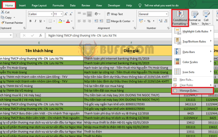
Step 4

If you want to change the color, just choose the Home tab on the toolbar. Then click on Conditional Formatting. A scroll bar appears, then choose Manage Rules.

How to alternate row colors in Excel

Step 5

Now, the Conditional Formatting Rules Manager dialog box appears. Select the formula you created earlier, then choose Edit Rule.

How to alternate row colors in Excel

Step 6

The Edit Formatting Rule dialog box appears, select Format… and then choose the color you want to change.

How to alternate row colors in Excel

Thus, the above article has instructed you on how to alternate row colors in Excel. Hopefully, this article will be helpful to you in your work. Wish you success!