How to apply a condition to a drop-down list in Excel

If you need more control over your Microsoft Excel drop-down list and want to display specific options based on a condition, you can follow these steps. Let’s assume you have personnel distributed across four regions: North, South, East, and West. Instead of working with all personnel, you want to filter them by region using two drop-down lists. The first drop-down will allow you to select the region, and the second drop-down will display only the staff members in that selected region. You can use your own data or download the provided .xlsx and .xls files for demonstration purposes.

Note: This technique only works with a matrix-style data set. While I will demonstrate the simplest technique here, there are more complex solutions available online. After implementing this solution, you may find that it’s not perfect but it is extremely easy to implement. If it doesn’t work for your specific scenario, consider using embedded drop-down controls as an alternative.

How to apply a condition to a drop-down list in Excel

Here’s a step-by-step guide:

1. Begin with a matrix-style data set, as shown in Figure A, which lists representatives in each of the four regions. The region names must be in alphabetical order from left to right.

2. To create the first drop-down list for selecting the region, follow these steps:

Select cell H2.

Go to the Data tab and click on Data Validation in the Data Tools group.

From the Allow drop-down, choose List.

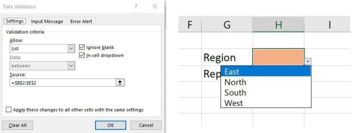
In the Source field, enter (or select) $B$2:$E$2 (Figure B).

e. Click OK.
Figure B: The drop-down displays the regions from row 2.

3. With the conditional drop-down in place, it’s time to create the dynamic drop-down that displays only the representatives from the selected region. Follow these steps:

Select cell H3 and repeat the steps from 2a to 2c.

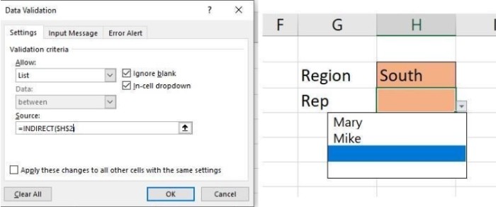
In the Source field, enter =Region $H$2 (Figure C). This formula references the value selected in the conditional drop-down cell H2.

c. Click OK.
Figure C: This drop-down uses the selected item in the conditional drop-down to determine its list.

Now, whenever you change the region in the conditional drop-down (cell H2), the representative drop-down (cell H3) will update accordingly. Remember to keep the conditional list of header text in alphabetical order. Additionally, note that the drop-down in Figure C has space for four items due to the presence of blanks. If you were to delete the name “Mary,” the first line would be blank, the second line would display “Mike,” and the third and fourth lines would remain blank. This is a trade-off when opting for an easy solution. For most users, these two drop-downs should work well enough.

For more Excel tips and tricks, consider reading our articles on mastering Excel with 56 essential tips, creating drop-down lists from another tab, adding color to drop-down lists, changing conditional formats on the fly, and combining Excel’s VLOOKUP() function with a combo box for enhanced searching. Additionally, you can explore our free PDF download compilations: “Build your Excel skills with these 10 power tips” and “13 handy Excel data entry shortcuts.”