How to Automatically Color Duplicate Data Cells in Excel
How to Automatically Color Duplicate Data Cells in Excel: In the process of working with Excel, we often face complex data and sometimes duplicates. One of the common causes of duplication is the habit of copy/pasting data multiple times into a spreadsheet. You need to find and remove duplicate data because just a few redundant data can affect the entire calculation result. So, how can you filter duplicate data in Excel quickly and accurately? This article will help you color the duplicate data cells in Excel to quickly identify the duplicated data cells.
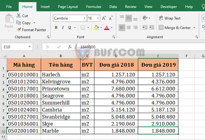
For example, we have a table of the prices of items in 2018 and 2019 as shown below. We want to compare the prices of products that have changed in 2019 compared to 2018 and those that have remained the same. To compare, please follow the steps below.
Step 1
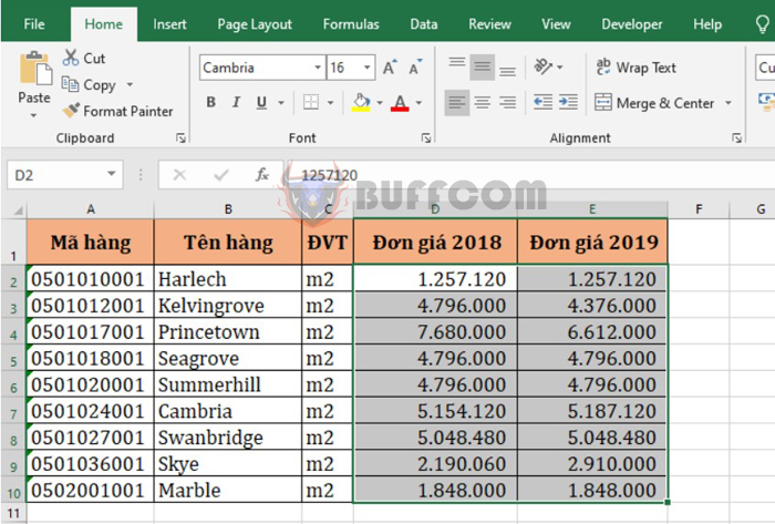
To compare prices between two years, first you need to highlight the entire data to be compared, which are the 2018 Price column and the 2019 Price column in the table.
How to Automatically Color Duplicate Data Cells in Excel
Step 2
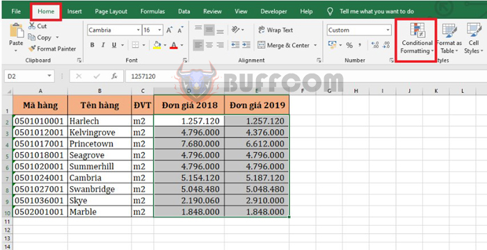
Next, select the Home tab on the toolbar. Then, choose Conditional Formatting under the Styles section.
How to Automatically Color Duplicate Data Cells in Excel
Step 3
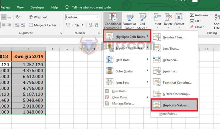
The scroll bar appears, select Highlight Cells Rules. Then, choose Duplicate Values.
How to Automatically Color Duplicate Data Cells in Excel
Step 4
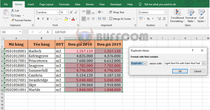
Now, the Duplicate Values dialog box appears. In the Format cells that contain section, choose Duplicate to highlight the cells with duplicate data. In the Values with section, you can click to choose a color, highlight border. Here are the color options for you to choose from:
- Light Red Fill with Dark Red Text: Highlight the cell with light red background and dark red text.
- Yellow Fill with Dark Yellow Text: Highlight the cell with yellow background and dark yellow text.
- Green Fill with Dark Green Text: Highlight the cell with green background and dark green text.
- Light Red Fill: Highlight the cell with light red background.
- Red Text: Highlight the cell with red text.
- Red Border: Highlight the cell with red border.
- Custom Format: Choose the color as you wish.
After you have finished choosing, click OK to complete. You can see that the products that have the same price in 2019 as in 2018 are highlighted.
How to Automatically Color Duplicate Data Cells in Excel
Step 5
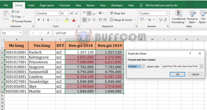
If you want to highlight cells with unique data, simply choose Unique in the Format cells that contain section. Then, click OK to complete. You can see that the products that have different prices in 2019 compared to 2018 are highlighted quickly.
How to Automatically Color Duplicate Data Cells in Excel
Therefore, this article has instructed you on how to automatically color duplicate data cells in Excel. Hopefully, this article will be useful for you in the working process. Wish you success!

