How to close parentheses for negative numbers in Excel
How to close parentheses for negative numbers in Excel: When working in an Excel spreadsheet, you may work with various types of data. When you want to distinguish negative cells from other types of cells, you should have Excel format that cell by enclosing it in parentheses or even highlighting it in red if it’s a negative number. This operation is not difficult and it also helps to present the data more visually and logically. This article will guide you through 2 ways to close parentheses for negative numbers in Excel. Let’s refer to the steps below.
Method 1: Close parentheses for negative numbers by eliminating the “-” sign
Step 1
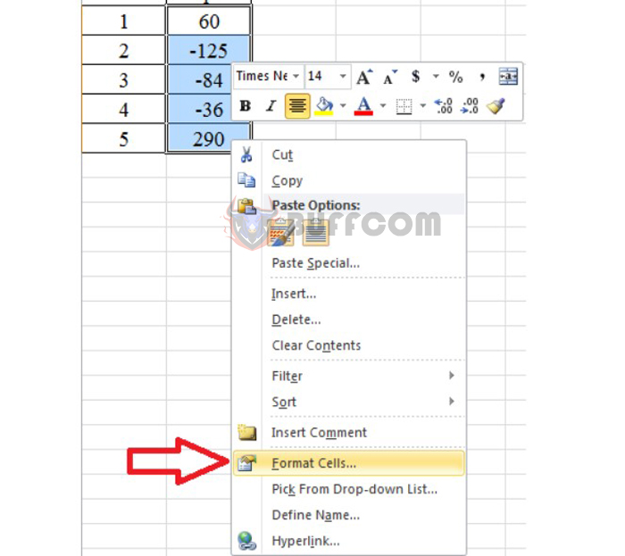
First, you need to enter a data table in Excel. Enter numbers into the table, including negative numbers. Next, highlight the column or area you want to format with negative numbers. Then, right-click on the highlighted area and select Format Cells…
How to close parentheses for negative numbers in Excel
Step 2
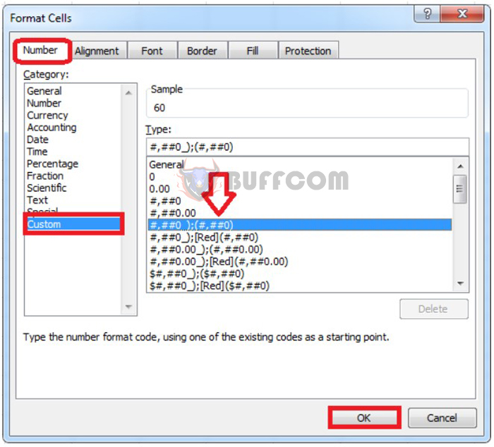
A Format Cells window will appear on the screen. Select the Number tab. Next, select the Custom item in the Category section. And when you look to the right of the Type section, find the format #,##0_);(#,##0), then press OK to use.
How to close parentheses for negative numbers in Excel
Step 3
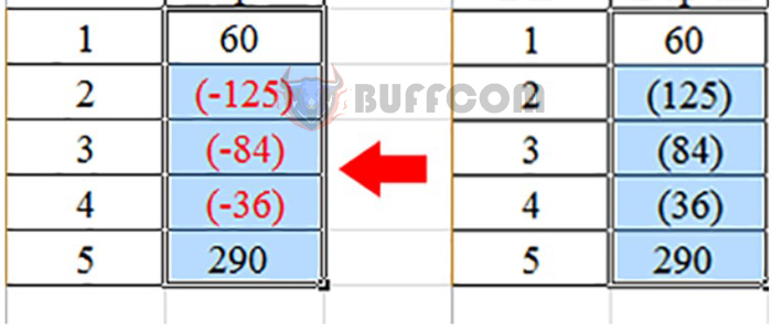
Immediately afterward, all negative numbers in the data table will be enclosed in parentheses and the “-” sign in front of them will disappear. Please see the image below:

How to close parentheses for negative numbers in Excel
Method 2: Close parentheses for negative numbers while keeping the “-” sign
Step 1
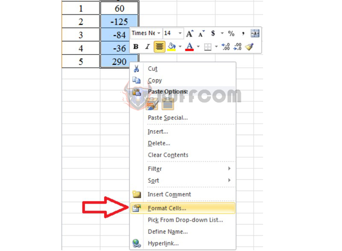
In case you want to highlight negative numbers in the data table while keeping the “-” sign in front of them, we proceed similarly. You also select the negative number range to be formatted, then right-click and select Format Cells….
How to close parentheses for negative numbers in Excel
Step 2
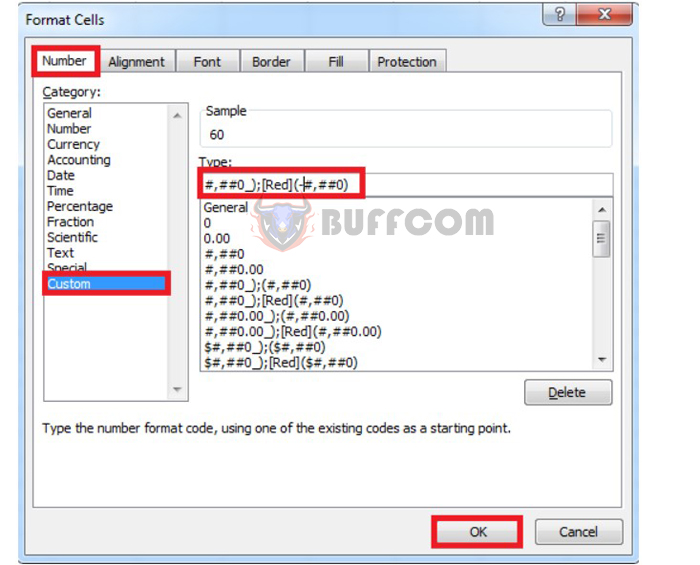
When the Format Cells window appears, select the Number tab. Here, in the Category section, we will select the Custom item. Looking to the right, you will find the format #,##0_);[Red](-#,##0) in the Type section. Once you have completed the operation, press OK to finish.
Note that if your Excel version does not have the format above in the Type section, you can copy and paste that format into the Type section. Then, press OK to execute.
How to close parentheses for negative numbers in Excel
Immediately afterward, the negative numbers will be highlighted in red on the screen. With this method, negative numbers in the data table have been converted to the enclosed format while still keeping the “-” sign.

How to close parentheses for negative numbers in Excel
In conclusion, formatting negative numbers in Excel can greatly improve the visual clarity of your data. By following the two methods outlined in this article, you can either eliminate the “-” sign and enclose the negative numbers in parentheses or keep the “-” sign and highlight the negative numbers in red. Both methods are simple to implement and will make your data easier to understand at a glance. So next time you’re working with negative numbers in Excel, try out these formatting techniques and see how they can benefit your work.


