How to Compare Two Columns in Excel Using Conditional Formatting
How to Compare Two Columns in Excel Using Conditional Formatting. In this tutorial, we will learn how to compare two columns in Excel 2016 using the Conditional Formatting tool. Conditional Formatting is a useful feature that allows you to visually analyze data and make your worksheets easier to interpret. It enables you to apply formatting based on cell values, such as colors, icons, and data bars. To compare two columns, we will create a conditional formatting rule.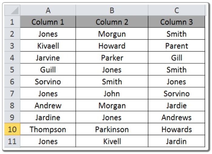
How to Compare Two Columns in Excel Using Conditional Formatting
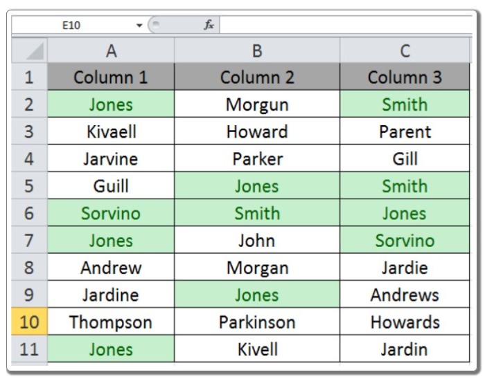
Let’s go through the steps to compare two columns in Excel using the following example. We have a list of names in three columns, and we want to identify the duplicate names.
- Select the cells that you want to apply conditional formatting to.
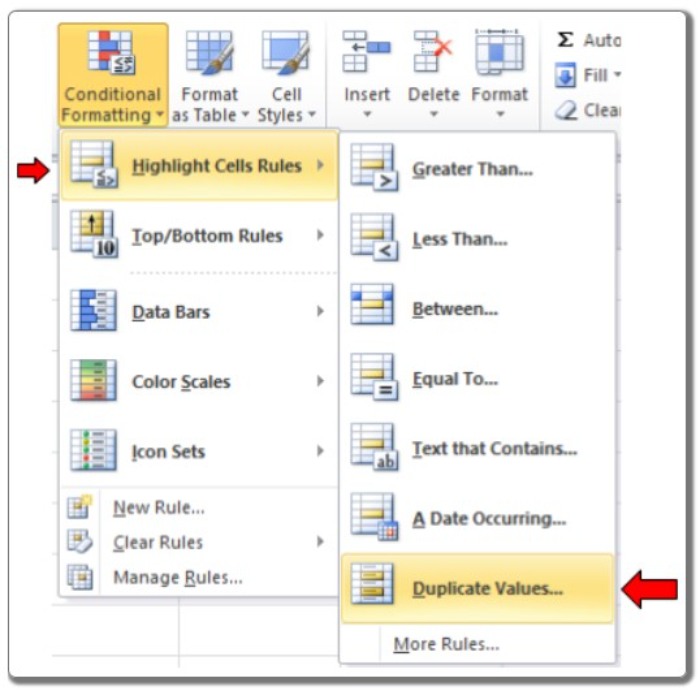
- Go to the Home tab, click on Conditional Formatting, and then choose Highlight Cell Rules.
- From the options, select Duplicate Values.
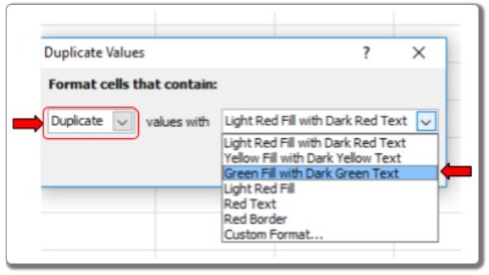
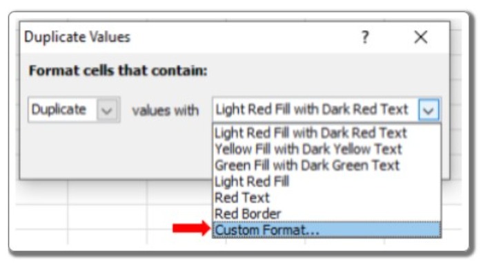
A dialog box will appear.
- In the dialog box, select “Duplicate” from the drop-down list, as shown in the snapshot above. Choose the formatting style you prefer, and click OK.
The duplicate values will be highlighted with a green fill and dark green text, as shown below.
You can further customize the highlight style and formatting by selecting the Custom Format option.
Using Conditional Formatting in Excel, you can easily compare two columns and identify any differences. For more information on Conditional Formatting, refer to other articles on this topic. If you have any queries or need assistance with Conditional Formatting, please leave a comment below, and we will be happy to help you.


