How to format negative numbers in parentheses using Format Cells in Excel
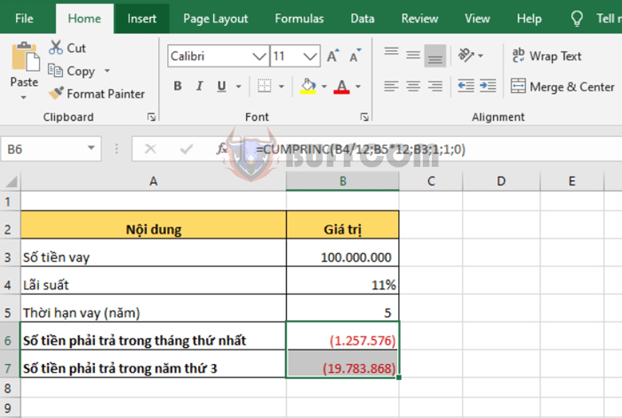
How to format negative numbers in parentheses using Format Cells in Excel: When working with Excel, there are times when you need to work with a large number of data types, so formatting negative numbers in parentheses is essential for easy identification. Follow the steps below to learn how to format negative numbers in parentheses using Format Cells in Excel.
Step 1
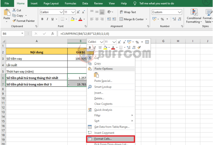
First, open the Excel file that needs to be reformatted with negative numbers in parentheses. Then right-click on the cells that need to be formatted with negative numbers in parentheses. The scroll bar appears, and you select Format Cells.
How to format negative numbers in parentheses using Format Cells in Excel
Step 2
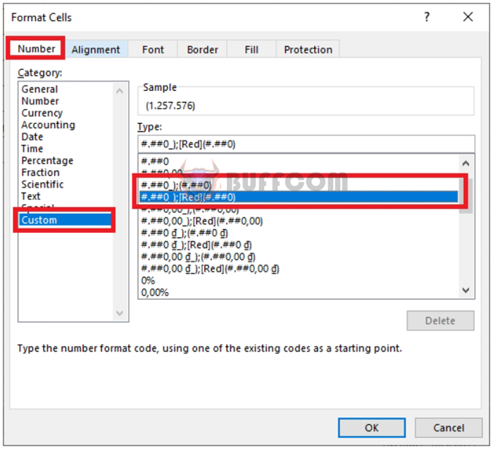
At this point, the Format Cells window appears. Select the Number tab. Then select the Custom option. In the Type section, you can choose the format to enclose negative numbers in parentheses as #.##0_);(#.##0) or #.##0_);Red if you want to highlight the number in red. Finally, click OK to complete.
How to format negative numbers in parentheses using Format Cells in Excel
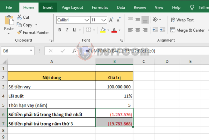
As a result, negative numbers will be enclosed in parentheses and highlighted in red as shown in the figure below.
 Step 3
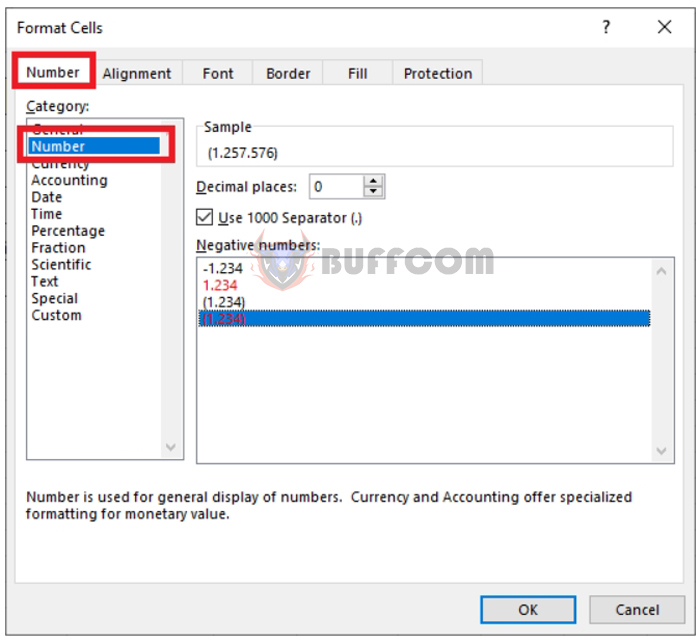
Alternatively, you can also choose to format negative numbers in parentheses by selecting the Number tab in the Category section of the Format Cells window. At this point, in the Negative Numbers section, you can choose the format for your numbers. You can also select a thousand separator by ticking the Use 1000 Separator option.
How to format negative numbers in parentheses using Format Cells in Excel
In conclusion, this article has guided you through the process of formatting negative numbers in parentheses using the Format Cells tool in Excel. Hopefully, this article will be useful to you in your work. Good luck!

